Managing a Commons

Preface

Epigram

For that which is common to the greatest number has the least care bestowed upon it. Every one thinks chiefly of his own, hardly at all of the common interest. —Aristotle (The Politics, Book II)

Freedom in a commons brings ruin to all. —Hardin (1968 p. 1245)

Overview

Learning Objectives

This chapter provides an introduction to management of a common-pool resource.

Background

Common Pool Resources

A common-pool resource is a resource that is rivalrous in use but limited in exludability. The classic example is a pasture commons. Although we may think of medieval England pasture commons, there are many modern examples. (The Open Spaces Society claims that there are over 7,000 registered commons in England alone.) Historically, the commoners had pasture rights in the commons (e.g., a village green, used for grazing).

William Foster Lloyd

In 1883, the 19-th century polymath mathematician, economist, and demographer William Forster Lloyd (1794 – 1852) provided perhaps the first clear statement of a problem with pasture commons. In Two Lectures on the Checks to Population, he observed:

If a person puts more cattle into his own field, the amount of the subsistence which they consume is all deducted from that which was at the command, of his original stock; and if, before, there was no more than a sufficiency of pasture, he reaps no benefit from the additional cattle, what is gained in one way being lost in another. But if he puts more cattle on a common, the food which they consume forms a deduction which is shared between all the cattle, as well that of others as his own, in proportion to their number, and only a small part of it is taken from his own cattle.

—Lloyd (1833) https://www.jstor.org/stable/pdf/1972412.pdf

Llody went on to explain the resuling tendency: resource exploitation in a commons would exceed the prudent level.

Hardin and Ostrom

In 1968, ecologist Garrett Hardin and termed this tendency “The Tragedy of the Commons”. In 2009, political economist Elinor Ostrom (1933–2012) shared a nobel prize in Economics for her institutional analyses of the functioning of actual commons, which often did not end up in tragedy. The claim that “a resource arrangement that works in practice can work in theory” is has been called Ostrom’s Law.

A Mathematical Analysis

In this section we give a high simplified mathematical analysis of the tragedy of the commons. (For an accessible analysis with more details, see Dasgupta (2005).) Let \(H=\sum_{i=1}^{N} H_i\) be the total size of the herd on the pasture. For our simple presentation, profit per cow (\(\pi\)) is linearly decreasing in herd density. This is a very simple formulation, but Overman and Scholtz (2002, p.283) find it useful empirically. Since the pasture size is a constant, profit per cow is correspondingly decreasing in total herd size.

\begin{equation*} \pi = a - b H \end{equation*}

with parameters \(a > 0\) and \(b > 0\). Consider first the profit maximizing herd size. Total profits are profits per cow times the number of cows, so profits are quadratic in herd size.

\begin{equation*} \Pi = \pi H = a H - b H^2 \end{equation*}

Recall from the properties of quadratic functions that the maximum will be at

\begin{equation*} H = \frac{a}{2b} \end{equation*}

with corresponding profits

\begin{equation*} \Pi = \frac{a}{4b} \end{equation*}

Now let there be multiple commoners, each choosing its own herd size, \(H_{i}\). Suppose we have two commoners.

\begin{equation*} \pi = a - b(H_1 + H_2) \end{equation*}

Then to maximize its own profit, each commoner chooses \(H_i\) to make \(\pi H_i\) as big as possible. Focus for a moment on the decision of commoner 1, whose profits are profits per cow times its herd size.

\begin{align*} \Pi_i &= \pi H_1 \\ &= a H_1 - b (H_1 + H_2) H_1 \\ &= a H_1 - b H_1 H_2 - b H_1^2 \end{align*}

This is at a maximum when

\begin{align*} 0 &= a - b H_2 - 2 b H_1 \\ H_1 &= (a - b H_2) / 2 b \end{align*}

Similarly,

\begin{equation*} H_2 = (a - b H_1) / 2 b \end{equation*}

This gives us a total herd size of

\begin{align*} H &= H_1 + H_2 \\ &= (a - b H_2) / 2 b + (a - b H_1) / 2 b \\ &= a/b - (H1 + H_2) / 2 \\ &= \frac{2a}{3b} \end{align*}

Corresponding, total profits are

\begin{align*} \Pi &= \pi H = a H - b H^2 \\ &= \frac{2 a^2}{9 b} \end{align*}

This is the tragedy of the unregulated commons: total herd size is larger than optimal. There is overuse of the common-pool resource. Total profits are correspondingly lower, as is each commoner’s profits. Yet it is a Nash equilibrium: neither commner has an incentive to reduce its own herd size.

This has the formal structure of a prisoner’s dilemma. If both commoners were to slightly reduce herd size, both could achieve higher profits. Yet if one commoner reduces herd size, the other has an incentive to increase herd size.

Biomass Growth

Biomass growth, including forage replentishment, is usually modeled as dependent on the current distance from a maximum biomass capacity.

\begin{equation*} V_{t+1} - V_{t} = \gamma(V_{t}) (V_{max} - V_{t}) \end{equation*}

Here \(\gamma\) determines the rate of growth. Two popular models of growback are

Partial Adjustment:: \(\gamma(V) = \bar{\gamma}\)
Logisitic Adjustment:: \(\gamma(V) = \bar{\gamma} V\)

In either case, the values of \(\bar{\gamma}\) fall between \(0\) and \(1\).

Logistic Growth

We need to represent the grow-back behavior of grass. Noy-Meyr (1978) and Paine et al. (2011) discuss a variety of plausible representations of the growth of green biomass. We select a representation that has been common since the work of Brougham (1955): the Verhulst-Pearl logistic growth function. (Logistic growth has been commonly applied to population growth since the work of Verhulst (1838) and Pearl (1927).) This function says that the growth rate is initially high but tapers toward zero as the land approaches its carrying capacity. Let \(\bar{V}\) be the green-biomass capacity of a patch of land. Then we can algebraically represent the growth rate (\(g\)) as

\begin{equation*} g = \bar{\gamma} (1 - V/\bar{V}) \end{equation*}

For example, if we set \(\bar{\gamma}=0.2\) then we have the following relationship between between the growth rate \(g\) and the current level of biomass \(V\) (relative to capacity).

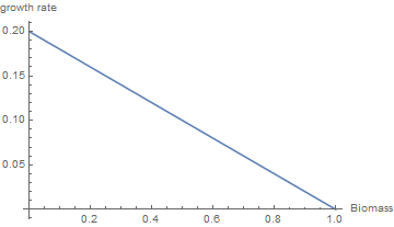
When \(V = 0\) then \(g = \bar{\gamma}\), the maximum proportional growth rate of green biomass. When \(V = \bar{V}\) then \(g = 0\), the minimum proportional growth rate of green biomass. The adjustment of \(V\) over next period will be

\begin{align*} V_{t+1} - V_{t} &= V_{t} g \\ &= V_{t} \bar{\gamma} (1 - V_{t}/\bar{V}) \end{align*}

implying that

\begin{equation*} (V_{t+1}/\bar{V}) = (V_{t}/\bar{V}) + \bar{\gamma} (V_{t}/\bar{V}) (1 - V_{t}/\bar{V}) \end{equation*}

We will write this as

\begin{equation*} v_{t+1} = v_{t} + \bar{\gamma} v_{t} (1 - v_{t}) \end{equation*}

and refer to \(v\) as relative biomass (i.e., relative to the biomass capacity \(\bar{V}\)). For example, if the maximum weekly growth rate is \(\bar{\gamma}=0.2\) and we start at 10% of capacity, then we have the following relationship between between time (measured in weeks) and the current level of biomass \(V\) (relative to capacity). Note that in the first 15 weeks we reach two-thirds of capacity, yet another 15 weeks leaves us short of full capacity. As full capacity is approached, the growth rate falls.

Valid Growth Rates

For this to make sense, we need the quantity in square brackets to be no more than one.

\begin{align*} 1 &\ge (V/\bar{V}) + \bar{\gamma} (V/\bar{V}) (1 - V/\bar{V}) \\ 1-(V/\bar{V}) &\ge \bar{\gamma} (V/\bar{V}) (1 - V/\bar{V}) \\ 1 &\ge \bar{\gamma} (V/\bar{V}) \\ \bar{\gamma} &\le (\bar{V}/V) \le 1 \end{align*}

So we will assume that \(\bar{\gamma} < 1\).

Sustainable Harvest

A weekly harvest is sustainable if each time we return to the field, we can again harvest the same amount. Given logistic growth of a field, what is the maximum sustainable harvest (relative to capacity)? Recall that

\begin{equation*} v_{t+1} = v_{t} + \bar{\gamma} v_{t} (1 - v_{t}) \end{equation*}

Equivalently, the biomass adjustment in a week is

\begin{equation*} v_{t+1} - v_{t} = \bar{\gamma} v_{t} (1 - v_{t}) \end{equation*}

The expression on the right is often called the logistic map. A harvest is sustainable if it is removing exactly the new biomass each time. For example, in the following figure, there are two levels of biomass that can support the given level of harvest. We can also see that we can harvest more than in the figure. The logistic map evidentally reaches a maximum at \(0.5\), so the maximum sustainable harvest is \(\bar{V} \bar{\gamma}/4\).

Calibration: Maximum Sustainable Harvest

We will approximate the maximum sustainable harvest of an acre of grazing land as \(200\) pounds per week. We will suppose an ungrazed acre could eventually grow to \(4000\) pounds of forage. This implies \(\bar{\gamma} = 0.2\). (Ideally this would be estimated for a real field.)

\begin{align*} 200 &= 400 \bar{\gamma}/4 \\ \bar{\gamma} &= 4(200/4000) = 0.2 \end{align*}

Carrying Capacity

We define the carrying capacity of a pasture as the maximum number of cows that can be sustainably fed by the pasture. In principle every patch can have its own sustainable harvest, but to keep things simple our patches will be uniform in this repsect. This means that to find the carrying capacity of the pasture, we need to divide its sustainable harvest by the consumption per cow.

We are going to work with crudely rounded numbers. We will approximate the weekly forage needs of a cow as \(400\) pounds. So we will need about 2 acres per cow.

Cows need about 4% of their weight in forage each day, which we round to 1/3 per week. We approximate cow weight as 1200 pounds. which mean a cow needs 400 pounds of forage per week.

With 25 grazing weeks per year, this is \(300\) pounds per week.

Geographical Extent

The land in our model will be represented by \(10,201\) patches laid out in a \(101 \times 101\) square. Each patch represents a tenth of an acre of land, so the total represents about 1.6 square miles of land. Although cattle need access to water and salt, we will concern ourselves only with grazing needs.

Since an acre of grazing land produces \(200\) pounds per week of forage, a patch produced \(20\) pounds per week.