PostScript Drawing for the Sciences
| Author: | Alan G. Isaac |
|---|---|
| Address: | Department of Economics American University Washington, DC 20016 |
| email: | aisaac@american.edu |
| update: | 2019-03-08 |
| since: | 2009-04-16 |
Abstract
Scientists and mathematicians often support their arguments with drawings. When these drawings are intended to illustrate very precise geometrical relationships, the PostScript page description language may be an appropriate tool. PostScript is a powerful, flexible tool for drawing, even for those who only learn the basics. A few lines of PostScript can often replace frustrating and tedious experimentation in a point-and-click environment. This booklet provides an introduction to scientific and mathematical drawing with PostScript. In order to clarify its advantages and drawbacks, we include some comparisons with a few other drawing languages or metalanguages.
Table of Contents
- Preface
- First Steps
- Programming in PostScript
- Transformations
- Dots
- Circles
- Rectangles
- Bézier Curves
- Coordinate Transformations
- More Programming in PostScript
- Adding Your Drawing to a Document
- Adding Text to a Drawing
- Clipping and Pattern Fills
- Other Stacks
- Encapsulated PostScript
- Images
- Conclusion
- Arrow Code
- Glossary of Useful Terms
- Other Useful Stuff
- Just for Fun: Yin Yang
- Standalone Pictures for Document Inclusion
- Appendix: Ghostscript
Preface
This booklet provides an introduction to the PostScript language, simple drawing with PostScript, and the production of complex PostScript drawings with simple scripts. In contrast with the typographical emphasis of most PostScript introductions, this booklet pays almost no attention to typography. Instead, we emphasize PostScript language features that are particularly useful for the production of simple but precise drawings. Our approach is visual and explanatory. Code listings are accompanied by illustrations and exercises.
Goals
Visual communication is part of science and mathematics. As a result, many excellent tools have evolved for producing charts. Many package can aid the production of excellent data charts, often with fine control over their appearance. Any decent computer-aided-design package can aid the production of precise technical drawings. For the most part, we will not be concerned with charts that are easily produced with such packages.
When choosing a drawing tool, one would like to pick the right tool for the task. The tool varies by task and background. Here are some core considerations:
- Can this tool produce the type of drawing you need?
- How quickly can you learn the basic use of this tool?
- How quickly can you produce the type of drawing you need with this tool?
- If you need to produce several related drawings, can you leverage work on one of them into progress on another?
When faced with the need to produce a technical drawing, the first stop will often be a good point-and-click vector drawing program. There are many good ones, both free and commercial. However the need for geometric precision or complex geometric shapes sometimes renders difficult or tedious the use of point-and-click drawing. At that point, the use of a drawing language (or metalanguage) comes under consideration.
There are many good drawing languages, both free and commercial. The ideal language will be easy to learn yet powerful, allowing flexibility in the illustration of precise geometric relationships. As we will see, the PostScript page description language meets these criteria.
The right tool can also depend on personality: some people find use of a drawing language more painful than searching through a myriad of drawing-tool menus, while others find menu search frustrating and truly enjoy programming. PostScript drawing is most likely to appeal to those who take some pleasure in the process of programming. It will also appeal to those who have perfectionist leanings when it comes to scientific drawing.
This booklet constitutes a self-contained introduction to PostScript drawing that is an adequate starting point for those who wish to add PostScript drawings to documents such as lecture notes, theses, dissertations, academic books, and journal articles. It also briefly discusses some more advanced topics and suggests resources for further study. Finally, for those already familiar with popular metalanguages such as TikZ or PyX, it offers some code comparisons. However, it does not offer instruction in the use of these alternatives. Only the PostScript language is discussed in any detail.
What is PostScript?
PostScript combines a general-purpose programming language with page-description functionality specialized for the static visual display of information. As a page description language, PostScript provide a rich collection of useful graphics commands.
A typical PostScript program provides a description of visual information: shapes and colors on a page. (Some of the shapes may be text.) To turn this description into a visual display, we need a PostScript interpreter. The interpreter converts our description (our code) into a representation on a computer screen or a printed page. Some printers have built-in PostScript interpreters. Other interpreters are available as software applications, which can be used for screen display or printing. Such interpreters are available for most platforms, including Windows, Mac, and Linux.
The examples in this booklet assume that you have access to a computer with an installed PostScript interpreter. If you need an interpreter, you have many options available, including the free and open source Ghostscript.
Background
In 1985, Adobe introduced the PostScript page description language [adobe-1999-plrm3] [p.5]. It soon became extremely popular for the production of professional drawings. For high resolution drawings intended for the inclusion in other documents, including academic books and journal articles, it quickly became the standard. Over time, this standard has been largely replaced by the Portable Document Format (PDF), which is heavily influenced by the PostScript language (but lacks PostScript’s control flow constructs). Since PDF is so closely related to PostScript, most drawings in PostScript can readily be converted to PDF.
PostScript output is produced by many software applications. Many spreadsheets, data-analysis packages, and scientific programming languages allow the creation of sophisticated data-driven or even functionally driven graphics that, as a rule, can be exported as PostScript. As a result, very few people have cause to write PostScript programs to create data-driven graphics. [1] There is also a plethora of drawing applications that support the export of PostScript graphics, and many of these applications require only a little point-and-click experimentation before the user can produce quite sophisticated drawings. [2]
| [1] | For those that do, [kunkel90gdps] provides an excellent introduction. However, first consider gnuplot, a free scientific plotting program that produces very flexible and high quality PostScript output. |
| [2] | Widely used vector graphics applications include Xfig, Jfig, Mayura Draw, Xara X, CorelDraw, and Adobe Illustrator.} |
Why then would anyone turn to the underlying PostScript language to produce a drawing? It is important ot be clear about this: often there will be no reason. The existing applications are fully adequate for many drawing purposes. Nevertheless, three basic reasons frequently arise: precision, speed, and fun. A fourth reason arises occasionally and can be crucial when it does arise: it may prove necessary to tinker with the PostScript produced by an graphics application---possibly to alter line characteristics or object placement---and even a novice's understanding of PostScript often makes this possible.
PostScript programming should therefore been seen as a complement to rather than a substitute for other approaches to the generation of vector graphics. The more precisely one wishes to render a simple drawing, the more likely it is that turning directly to the PostScript language will prove valuable. PostScript excels at the precise representation of geometric relationships. Since PostScript is a page description language that is particularly simple in structure, precise geometrical relationships that can be difficult to produce accurately in a point and click environment often require only a few minutes of PostScript programming.
To illustrate this claim, compare the ease of production of Equilateral Triangle or Circumscribed Circles below with the difficulties in achieving precise equivalents in your favorite “point-and-click” vector graphics application. Or consider the ease with which the techniques used in Equilateral Triangle can be generalized to the production of regular polygons of any dimension. Finally, a little PostScript programming can produce results that are visually quite exciting, so it is impossible to neglect the fun involved.
Some Alternatives
In the 1990s, PostScript was an alternative to the LaTeX picture environment. The picture environment was very simple to use, but sometimes a more powerful drawing language was needed. [3] PostScript provided this power, and learning to draw in PostScript requires surprisingly low effort. One can very quickly learn to produce complex but precise drawings in the powerful PostScript page description language---nearly as quickly as one can learn the LaTeX picture environment and more quickly than one can learn precise drawing in many point-and-click environments.
| [3] | The LaTeX picture environment is documented by [lamport-1994-latex] [appendix~C.14.1].
It offers a powerful mechanism for the placement of mathematics on a drawing.
The LaTeX drawing constructs are useful but very limited when compared with PostScript;
LaTeX drawings are also less portable (unless first converted to PostScript or another format).
If use of LaTeX and PostScript is a given,
the advantage of LaTeX in typesetting mathematics is easily combined with the power of PostScript drawing:
just \put{} an included EPS graphic into a LaTeX picture environment,
be careful about your units (PostScript points are the same as TeX big points),
and then \put{} the math into the picture environment as well.
(For a more elegant solution, see the PSfrag package.) |
However, LaTeX has also evolved and now supports the Portable Graphic Format (PGF), which has very strong drawing capabilities. These capabilities are further strengthened by a widely use library of macros for PGF, which is called TikZ. Together, TikZ can make complex drawing, including the placement of text, simple and convenient. This comes at some cost in complexity: the PDF/TikZ manual has more than 1000 pages. Nevertheless, simple basic constructs are often adequate even for complex drawings. Furthermore, PGF can produce either PostScript or PDF output, so it can be considered to be a PostScript metalanguage. This booklet provides some TikZ examples for comparison.
Essentials
While vector drawing applications can be expensive, tools for PostScript programming are available for free. However the true cost of producing any drawing will have little to do with monetary cost, since drawing can be very time consuming no matter what environment is chosen. For most economists, drawing by means of PostScript programming will be worthwhile only in those circumstances where simple programs can produce results that would require time-consuming point-and-click experimentation in a vector graphics application. After dealing with a few essentials and introducing some basic considerations, this booklet will provide a few examples of such programs.
To create and view PostScript drawings on a computer, you need only a text editor and an “interpreter” supporting screen display. [4]
| [4] | Many printers include a PostScript interpreter (or a clone), but even people with access to such a printer will find it helpful to be able to view their drawings on screen.} |
The inexpensive options for interpreters that permit onscreen viewing are limited but high quality. The standard is the free Ghostscript interpreter, which allows previewing and printing PostScript files on many platforms. [5]
| [5] | Many Ghostscript users will also want a graphical interface to Ghostscript, such as GSView (for Windows/Linux/OS2), MacGSView for the Mac OS, and GhostView for Unix and VMS. Windows users may be interested in the small, fast RoPS interpreter, which has a free LanguageLevel 1 version. Serious PostScript programmers may profit from PSAlter's helpful debugging facilities.} |
As for text editors, this booklet focuses on very simple examples, for which you can use the default editor on your computer (or even a word processor, if you remember to save what you type as ASCII text). [6]
| [6] | Windows operating systems include NotePad, Unix and related systems usually include vi, and Macintosh operating systems usually include TeachText. These will be adequate for our simple experiments. |
Finally, for anyone intending to go beyond the most casual use of PostScript, I strongly recommend downloading [adobe-1999-plrm3], which is a precise yet usually readable reference manual.
Resources
There are many tutorials and books introducing PostScript. Here we list just a few, with short annotations. Many are available online. (See the reference section for the URIs I am aware of.) Anyone who finds the present booklet to be useful will undoubted find Bill Casselman’s wonderful book to be useful as well.
Books
- [adobe-1999-plrm3]
- The “red book”. Absolutely crucial reference manual; comprehensive yet accessible. Includes an alphabetical list of PostScript operators. Archived at http://partners.adobe.com/public/developer/ps/index_specs.html
- [heck-2005-wp]_
- A useful online tutorial. It is more lengthier and more advanced than most online tutorials, but it starts with the basics. https://staff.science.uva.nl/a.j.p.heck/Courses/Mastercourse2005/tutorial.pdf
- [casselman-2005-cup]
- A wonderful discussion of mathematical drawing with PostScript. Highly recommended.
- [adobe-1988-plpd]
- The “green book”. Not quite so useful as the tutorial, but still contains useful ideas. Archived at http://partners.adobe.com/public/developer/ps/sdk/index_archive.html
- [adobe-1985-pltc]
- The “blue book”. Accessible, with many examples. Archived at http://partners.adobe.com/public/developer/ps/sdk/index_archive.html
- [mcgilton.campione-1992-psxmpl]
- PostScript by Example emphasizes examples, like the present booklet. An early but still very enjoyable introduction to PostScript drawing.
- [reid-1990-thinking]
- Thinking in PostScript is good guide quickly learning PostScript for those who already program.
- [braswell-1991-insideps]
- Inside PostScript focuses on technical interpreter details;
primarily of interest for implementation details of the Adobe PostScript interpreter.
Small translations may occasionally be required by GhostScript users
(e.g., translate
.errorassignalerrorand=printas=only.) - [roth-1988-rwps]
- The “orange book”: Real World PostScript collects diverse and instructive PostScript applications.
Websites
- PostScript Tutorial:
- https://github.com/luser-dr00g/pstut/wiki
An unusually useful tutorial written by Josh Ryan (luser drOOg),
the creator the the
xpostPostScript interpreter (https://github.com/luser-dr00g/xpost ; license: BSD). - comp.lang.postscript
- PostScript Users Group: https://groups.google.com/forum/#!forum/comp.lang.postscript Frequented by helpful experts.
- ehandler.ps
- Error handler for troubleshooting PostScript errors. Available (2016-08-20) at http://www.adobe.com/support/downloads/detail.jsp?hexID=5396, along with some usage instructions.
- David Maxwell's online PostScript manual
- http://www.ugrad.math.ubc.ca/Flat/ps-toc.html
- PostScript Basics
- http://www.prepressure.com/ps/whatis/PSlanguage.htm
- Luc Devroye’s PostScript page
- links to many utilities. http://luc.devroye.org/postscript.html
- Konrad Parker’s LegoBrot
- builds three-dimensional fractals http://www.kfish.org/fractals/legobrot/
- Peter Weingartner’s “A First Guide to PostScript”
- http://www.cs.indiana.edu/docproject/programming/postscript/postscript.html
- MIT PostScript archive
- https://stuff.mit.edu/afs/sipb/contrib/postscript/ Interesting PostScript examples.
- Jim Land’s “Internet Resources for PostScript and GhostScript”
- A metalist of resources. http://www.inkguides.com/postscript.asp
- John Deubert’s Acumen Training
- Extensive resources, including theAcumen Journal http://www.acumentraining.com/acumen_journal.html
publishes PostScript code examples. Don Lancaster’s Guru’s Lair
Full of resources, including his PostScript Library http://www.tinaja.com/post01.asp
- WPS
- A PostScript and PDF interpreter for HTML 5 canvas; you can now use PostScript as a drawing language in web pages http://logand.com/sw/wps/index.html
- Resources for the PostScript® language
- anastigmatix.net provides interesting PostScript resources, including sorting and order statistics http://www.anastigmatix.net/postscript/Order.html
- PostScript FAQ
- https://en.wikibooks.org/wiki/PostScript_FAQ Includes GhostScript-specific details.
First Steps
This booklet discusses the creation of PostScript programs that describe a chart that can fit on a single page. We refer to these as PostScript drawings. (Later on, we discuss how to embed PostScript drawings in larger documents.) There are two basic steps in creating a PostScript drawing: first construct a path, then paint it. Almost all our effort will be spent on path construction.
Canvas Coordinates
Locations on the page are designated in a familiar fashion: we use standard Cartesian coordinates. When we start drawing, the location \((0,0)\) is at the lower left corner of the page. Increases in the first coordinate produce more rightward locations; increases in the second coordinate produce more upward locations. The default unit of measurement in PostScript is the printer DTP point, which is 1/72 inches. So an 8.5 inch by 11 inch page measures 612 points by 792 points. We illustrate this in PostScript Page (Letter Size) by labeling a few locations on an image of a letter-size page. In geometry, dimensionless locations are usually called points, and these must not be confused with the DTP point unit of measurement.
PostScript Page (Letter Size)
The Process of Drawing
We create a PostScript drawing with PostScript operators. A PostScript operator may require one or more operands. For example, PostScript drawings often begin with the moveto operator. The moveto operator needs two operands, which provide the coordinates of a position on the page. So x0 y0 moveto moves the current point of our drawing to the position \((x_0,y_0)\). Note that the operands precede the operator. (PostScript is a stack-based languaged; we will explain this later.)
Consider the construction of a line segment between any two locations on the page. We can characterize a line segment by the coordinates of the two endpoints. To construct the corresponding PostScript path, we can use the moveto operator to move to one endpoint and then the lineto operator to construct a line segment to the other endpoint. (A PostScript operator will often have a name that resembles an ordinary language description of its function.) Like the moveto operator, the lineto operator needs two operands: the coordinates of a position on the page. It constructs a line segment from the current point to the coordinates specified by its operands, and the coordinates become the new current point of our drawing. We are now ready to under the following lines of PostScript.
x0 y0 moveto
x1 y1 lineto
The first line of code moves the current point of our drawing to the position \((x_0,y_0)\).
The second line of code constructs a line segment from there to the position \((x_1,y_1)\),
which becomes the new current point for our drawing.
(Of course to use these lines of code,
we need numerical values for x0, y0, x1, and y1.)
With just this information, you could readily construct any figure composed of straight line segments, as long as you know the coordinates of the endpoints of each line segment. The ability to draw straight lines encompasses a surprising number of drawing needs. Even plots of non-linear functions are frequently drawn as a sequence of short line segments.
Our discussion so far has focused on absolute coordinates. We can also work with relative coordinates. We often find it useful to construct paths using relative movements, and this is the basis of a second approach to line segment construction. For example, a line segment can be characterized by an endpoint and a displacement from that endpoint. To construct the corresponding PostScript path, we can again use the moveto operator to move to one endpoint, but then we can use the rlineto operator to construct a line segment to the other endpoint. The rlineto operator needs two operands: the horizontal and vertical displacements relative to the current point on the page. These determine the coordinates of the other end of the line segment. We are now ready to under the following lines of PostScript.
x0 y0 moveto
dx dy rlineto
The first line of code moves the current point of our drawing to the position \((x_0,y_0)\). The second line of code constructs a line segment from the current point to the position \((x_0+dx,y_0+dy)\), which then becomes the new current point for our drawing.
So far we have been focusing on path construction. Recall that there are two basic steps in creating a PostScript drawing: first construct a path, then paint it. We will not be able to actually view a constructed line segment until we add ink, as it were. We can use the stroke operator to do this.
Exercise
Launch Ghostscript (or an alternative interactive viewer) and enter the commands:
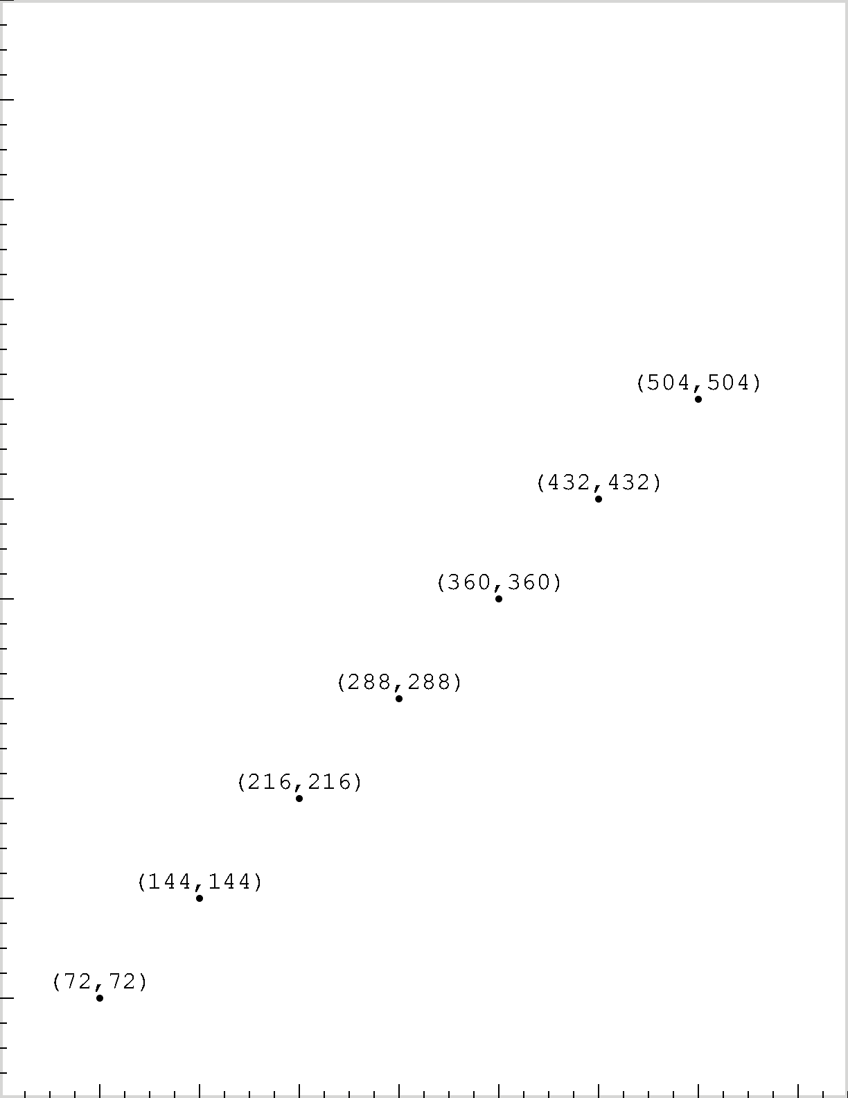
72 72 moveto
288 288 line
stroke
Do you see what you expect to see?
Displaying Your Drawings
When working with a very small amount of code,
it is quite feasible to simply enter PostScript at the Ghostscript command line.
However, we generally want to store our code in an ASCII text file,
which we can repeatedly modify and run.
Here is what the contents of such a file could look like.
Copy the following lines into a new text file, say project01.ps,
and save the file to disk.
(In the next section, we offer a detailed discussion of this code.)
%!                   %special comment (file is PostScript)
72 72 moveto         %set starting point for path
234 648 rlineto      %construct first line segment
234 -648 rlineto     %construct second line segment
closepath            %construct final line segment
4 setlinewidth       %set the line width to 4 points
stroke               %paint the constructed triangle
showpage             %render the drawing
You can use a GUI application (such as GhostView)
to interactively choose a printer and print your drawing.
Or you can send the file straight to a PostScript enabled printer.
If you are sending your file to a printer,
the showpage operator will produce (eject) a printed page.
So we conclude our drawing with the showpage operator.
Here we illustrate printing from a Windows computer.
If you have a PostScript enabled printer,
to print project01.ps,
you can give the following command from the command line:
copy project01.ps lpt1:
However, most of the time we “print” our drawing to a monitor screen.
In this booklet,
we assume you are using the free and open source Ghostscript.
At the Ghostscript command prompt,
enter (project01.ps)run. [7]
| [7] | Give a full path to your program file.
On Windows, backslash separators can be doubled,
or you can use forward slashes:
(c:\\psprojects\\project01.ps)run or
(c:/psprojects/project01.ps)run.
Ghostscript locks the file while running it.
If your file contains an error,
Ghostscript does not release the lock.
However, if you use the save operator before running your file,
then using the restore operator afterwards will release the lock.
So consider running your program like this:
save (c:/psprojects/project01.ps)run restore. |
After completing Isoceles Triangle (below),
use your PostScript interpreter to view project01.ps.
You will see a triangle, as in Isoceles Triangle.
(For your convenience,
we display the drawing as it would appear on a sheet of letter paper,
with the page boundaries added as a light gray outline.)
Project: Isoceles Triangle
The drawings in this booklet are produced by simple PostScript programs,
which are ASCII text files containing only a few lines of PostScript code.
The % character delimits a single-line comment.
Anything following the % character is a comment,
which will be ignored when we run our program.
Conventionally, each PostScript program begins with a special comment:
a single line containing the two characters %!. [8]
| [8] | This is not required by the PostScript language specification, nor is it required for rendering the examples in this booklet using Ghostscript. However, many applications, printers, and printer controllers recognize this as a special comment indicating that they are dealing with a PostScript file. For example, a printer with PostScript capability may rely on this special comment to determine whether to load a PostScript interpreter or a PCL interpreter. The PCL interpreter would print the source code rather than our drawing. |
Here we will explore the details with an extremely simple drawing that is a classic first project in PostScript: an isoceles triangle. In order to emphasize the precision of PostScript drawings, we will be very specific about certain details. We will assume a letter size page (8.5 inches by 11 inches). We will construct that largest isoceles triangle possible, subject to the contraint that the constructed path is within a one inch margin. [9] For example, we will place the first vertex of the triangle one inch (i.e., 72 points) from the bottom and one inch from the left side of our sheet of paper.
| [9] | For simplicity we are currently discussing only the location of the constructed path and not the width of the line when we stroke it. The basics covered in this section are covered in all good introductions to PostScript drawing, including [adobe-1985-pltc] [ch.3,6] and [mcgilton.campione-1992-psxmpl]. |
Begin this project by creating a new ASCII text file with any text editor.
We might as well call it project01.ps.
Next we enter the program code listed above.
Recall that we want to construct a triangular path, and then paint it.
In this example,
we begin our path construction with the instructions 72 72 moveto,
which sets the beginning of the path to the point \((72,72)\).
Next we construct two line segments:
the first side with 234 638 rlineto,
and the second with 234 -638 rlineto.
We construct the remaining side in a special way:
we use the closepath operator,
which constructs the line segment from our current point
to our starting point (for this path).
That completes our path construction.
Next we need to paint the constructed triangle. We will do this with the stroke operator, but first we use the setlinewidth operator set a nice thick line width of 4 points.
At this point we have completed our page description. We are done with our PostScript drawing. If you are using an interpreter that displays on screen each path as it is painted, you will see your triangle on the screen. To indicate that this is the end of our page description, we use the showpage operator. (More on this later.) Congratulations. You have produced your first PostScript drawing!
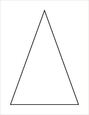
Isoceles Triangle
Project 1: Line by Line
We will now consider our first PostScript program in more detail. The first program line is simply a special comment that conventionally declares the file to be a PostScript program file. We end our program with the showpage operator, which displays the page. Between the first and last lines we find the two basic steps in creating a PostScript drawing: we first construct a path, and we then paint it. We have already briefly discussed these steps, now we provide additional detail.
Note that as an alternative to storing this code in a program file, you can enter it line by line at the Ghostscript command line. This can be convenience for experimentation.
Path Construction
To begin constructing a path, we need to pick a location where we will start drawing. We now make an arbitrary choice: we pick \((72,72)\) as the starting position for the path we wish to construct. We move the current point to there with the moveto operator. So the second line of our program is 72 72 moveto, which instructs the interpreter to make the position \((72,72)\) the current point of the path we are constructing.
The next step is to construct a line segment from \((72,72)\) to another position on the page. We use the rlineto operator, which consumes two operands that are the relative movements in the horizontal and vertical directions. We want to move 3.5 inches to the right and 9 inches up. Recalling that there are 72 points per inch, this is 234 points to the right and 648 points up. So we construct our first line segment with 234 648 rlineto. This instructs the interpreter to construct a line segment from the current point \((72,72)\) to the position \((306,720)\) based on the relative movement that we specified: \((72,72) + (234,648) = (306,720)\). This then becomes the new current point of the path we are constructing.
We still need to add two more line segments to our path. The fourth line of the program instructs the interpreter to construct a line segment from our current point \((306,720)\) by moving right by 234 points and down by 648 points, producing a new current point of \((306,720) + (234,-648) = (540,72)\). In the fifth program line we complete our construction of the triangle: the closepath operator constructs a line segment from the current point of our path to the starting point of our path (as determined by our initial moveto command). In our case, the current point when we give the closepath command is \((540,72)\), and we began our path at \((72,72)\). This completes the construction of our triangle, and we are ready to paint it.
Painting
Constructing a path does not in itself give us anything to view. We need to “paint” the path to produce a drawing. For our first painting operation, we will use the stroke operator. The stroke operator may be thought of as putting “ink” on the path we have constructed: until we stroke our path, there is nothing to view.
A natural question arises at this point: what determines the color and line width of the stroked path? When we stroke a path, the line width and color are determined by the current graphics state. PostScript provides default values but allows us to change these. In our program, we change the line width from its default of 1 point to a wider 4 points. We keep the default color, which is black. The section on Grayscale will show how to change the color.
Note that all of our path construction and painting code could have been placed on a single line. Instead we placed an easily interpretable code snippet on each line, and we included a helpful comment with each code snippet. This makes our code more readable and easier to debug.
Once we construct the path and stroke it, we use showpage to render what we have drawn. This instructs the interpreter to render everything we have painted on the page. [10] We can view the triangle illustrated in Isoceles Triangle.
| [10] | The showpage operator also tells a PostScript printer to eject the page. |
What if we had wanted a filled triangle rather than a stroked triangle? We need change only one line of our PostScript program: replace the stroke operator with the fill operator. This fills our triangle with black. (Try it.) We can fill our triangle with other colors (or even patterns): see sections on Color_ and on Clipping and Pattern Fills.
Line Width :code:````
The default line width is one unit; the default unit is one point. PostScript allows direct control of the line width with the setlinewidth operator. For example, 4 setlinewidth sets the line width to 4 units (which is 4 points, by default).
As an analogy, we might say that a path can be stroked with a “pen nub” of any width we desire. The setlinewidth operator does just what it's name suggests: it sets the width of the lines drawn when the path is stroked. This operator takes a single numerical operand: a line width in the current units of the user space. We will talk about changing those units in Transformations, but the default unit of measurement is one point.
As an exercise, choose a ten point wide “pen nub” by changing the line width with 10 setlinewidth before you stroke the triangle. View the result, and note that half the width of the “ink” falls on each side of the path. Note that the setlinewidth operator affects all subsequent stroke commands until you reset it.
Relative vs Absolute Positions
We have explored the use of the moveto and rlineto operators in path construction. PostScript also provides the rmoveto and lineto operators. The moveto and lineto operators are for absolute movement, which is movement to specified coordinates in the user space. The rmoveto and rlineto operators are for relative movement. Relative movement is relative to the current point. The operands of the rmoveto and rlineto operators are not positions but are rather the displacements (dx,dy) relative to the current point.
From any current point, we can use the rmoveto operator to make a relative movement (dx,dy) to the beginning of a new subpath_. Similarly the rlineto operator also takes as operands the horizontal and vertical displacements (dx,dy) relative to the current point. Reliance on relative movements can be particularly useful if we wish to construct the same object at multiple positions on the page: using relative movements allows us to reuse our code at various positions.
As an example, our code constructs our first side of our first triangle as 72 72 moveto 234 648 rlineto. We could instead use only absolute movement and write 72 72 moveto 306 720 lineto.
Key Lessons
Much of what we need to know in order to draw with PostScript is contained in our first simple program. Note in particular our use of units of measurement, a coordinate system, and postfix syntax.
By default, the basic unit of measurement is one point. [11] There are exactly 72 points per inch. So an 8.5 inch by 11 inch sheet of paper is 612 points by 792 points. The coordinate system is a standard Cartesian coordinate system, with the origin in the lower left corner of the page. The location \((72,504)\), for example, is one inch (72 points) to the right of the origin and 7 inches (504 points) above it.
| [11] | This is a unit of measurement. Do not confuse it with the “points” of the Cartesian coordinate system, which are dimensionless positions.} |
As for the syntax, you probably noticed that we always state a position before doing something with it (e.g., moving to it, or constructing a line segment to it). More generally, the PostScript interpreter should always encounter an operator after the operands required by that operator. For this reason, we say PostScript uses a postfix notation: an operator follows its operands. First you state the operands; then you state operator that will use these operands. We say that you push the operands onto the operand stack, where they can be found by the operator. [12]
| [12] | Some readers will be familiar with postfix syntax from the use of calculators that rely on reverse polish notation. I offer the online calculator PSCalc as a quick way to get familiar with some basic PostScript operators.} |
PostScript syntax is discussed in additional detail in Programming in PostScript.
Readers with programming experience will have noticed that we do not compile a PostScript program into an executable file that can run on a computer without an interpreter. We always use a PostScript interpreter to run our programs. We say that PostScript is an interpreted language.
We have already acquired enough tools to construct any drawing whose constituents are line segments, as long as we can specify the endpoints of each line segment. This includes graph axes, arbitrary polygons, linear functions, or even line graphs of time series. This drives home the flexibility of the PostScript page description language: after a few minutes of exposure, one is ready to create very complex drawings with great precision. This simplicity has another advantage: most vector drawing programs rely on proprietary and undocumented formats, whereas your own PostScript drawings will rely on a fully documented open standard and---since your code is simple ASCII text---will always be readable with any text editor. Of course one can usually export PostScript from a drawing application, but that PostScript is often filled with obscurities. Hand coded PostScript drawings will generally be easy to understand, easy to modify, and readily transportable. Finally, even if you once manage to produce a complex drawing in a vector drawing application, you may be unable to recall the sequence of actions that produced the drawing. In contrast, your PostScript program will always document the steps you took to produce a drawing, and you can add explanatory comments to enhance the value of this documentation.
Metalanguages: Isoceles Triangle
PyX: Isoceles Triangle
Before attempting any of the projects with PyX, be sure to read the PyX FAQ.
PyX is heavily influenced by the PostScript drawing model. When creating short, simple drawings, it is likely to be relatively verbose. However it is extremely flexible and makes hard things easy. Furthermore, it is easy to use PyX to augment and annotate existing PostScript drawings, as we will see later.
There are a few suprising differences from PostScript behavior. Probably the most unexpected difference is that the default line width is 0.2 centimeters, which is just over half of the PostScript default of 1 point. (This was chosen as a more suitable companion to the TeX fonts.) We will not bump up against this peculiarity as long as we always explicitly set the line-width in our drawing, which is a good practice in any case.
Another difference is the default unit is 1cm rather than 1pt. We will address this by always resetting the default unit.
import pyx
pyx.unit.set(defaultunit='pt')
We will implement our first project using PyX
in a way that emphasizes parallels to PostScript.
We begin by importing the pyx package.
To keep things as close as possible to our PostScript code.
we set the default unit of measurement to 1 point.
(See above.)
After that,
we construct the path and paint it.
The parallels to our PostScript code are extremely close,
but note two key differences.
Whereas our PostScript code is itself a page description,
which can be rendered by a PostScript interpreter,
our PyX code is not.
After constructing a path in PyX,
we create an abstract canvas on which to paint the path.
This canvas object has a writePSfile method,
which we then use to create a PostScript file.
(PDF and SVG output are also possible.)
So we use PyX to generate the PostScript
that we will use an interpreter to display.
Here we take the following approach. A PyX path is essentially a list of pathitems. Like a list, we can append to it or extend it. Once we have built up the path that we wish, we can paint it on a canvas.
Whereas in PostScript you would transform the user space and construct paths in the transformed space, in Pyx you effectivelyconstruct paths in a fixed user space but you can then transform these constructions.
#construct the path
isoceles_path = pyx.path.path(
pyx.path.moveto(72, 72),
pyx.path.rlineto(234, 648),
pyx.path.rlineto(234, -648),
pyx.path.closepath()
)

#create a canvas to paint on
cvs = pyx.canvas.canvas()
#paint the path on our canvase
cvs.stroke(isoceles_path, attrs=[pyx.style.linewidth(4)])
#write a PostScript file
cvs.writePSfile('pyx-isocleles.ps')
TikZ: Isoceles Triangle
TikZ drawing can be done in a tikzpicture environment.
Like PyX, the default unit of measurement is 1cm.
For comparability we will reset this when we draw.
The TeX big point (bp) is the same as the
PostScript point: 1/72 inch.
\begin{tikzpicture}[x=1bp,y=1bp]
\path[draw,line width=4bp] (72,72) -- ++(234,648) -- ++(234,-648) -- cycle;
\end{tikzpicture}
- Useful background:
- https://www.sharelatex.com/blog/2013/08/27/tikz-series-pt1.html
Mathematica: Isoceles Triangle
In comparison to TikZ and PyX,
the Mathematica drawing language is much less influenced by PostScript.
Mathematica currently has a limited concept of movement by relative displacement along a path. [13]
However, we can represent relative movement by doing vector addition.
Here we use the Accumulate command to accumulate our relative changes.
pts = Accumulate[{{72, 72}, {234, 648}, {234, -648}}]
pth = JoinedCurve[Line[pts], CurveClosed -> True];
Graphics[{Thickness[4/612], pth},
  PlotRange -> {{0, 612}, {0, 792}},
  ImageSize -> {612, 792}
]
| [13] | However, see the discussion of AnglePath in Equilateral Triangle. |
Mathematica constructs drawings from “graphics objects”,
including lines and joined curve segments.
Once we have our triangle vertices,
we can construct connecting line segments with the Line command,
and then use JoinedCurve with the CurveClosed option
to create a closed path.
The Mathematica drawing model does not use the notion of a canvas.
Graphics will automatically be given a bounding box that is intended
(usually successfully) to accommodate the entire drawing.
To mimic drawing on a full letter-page canvas,
we can use the PlotRange command,
setting a plot range corresponding to the PostScripts letter-page userspace coordinates.
Controlling the linewidth in our figure poses a special challenge.
Mathematica has two basic ways to control line width:
Thickness, and AbsoluteThickness.
Thickness is relative to the width of our graphic.
Absolute thickness is measured in points,
which initially sounds promising.
However, the Mathematica coordinate system is not in points.
(In fact, it is not in any fixed unit of measure.)
The actual size of the graphic is controlled by a separate ImageSize option,
which is measured in points.
So in order to get exactly what we want,
we first specify an image size chosen to match our plot range,
and then we also specify a line thickness relative to our plot range.
Explicit path construction did not really enter the language until version 8,
with the introduction of the JoinedCurve and FilledCurve primitives.
Here is a more traditional approach to this drawing.
(You may use the specialized Triangle command instead of Polygon.)
t1 = Polygon[pts];
t1style = Directive[EdgeForm[Thickness[4/612]], FaceForm[]];
Graphics[{t1style, t1},
  PlotRange -> {{0, 612}, {0, 792}},
  ImageSize -> {612, 792}
]
One other thing is worth noting.
Mathematica has a rather good ability to parse simple PostScript
and produce a Mathematica equivalent.
This PostScript drawing is very simple,
so we could simply create a string from our PostScript commands
and use the ImportString command to produce our drawing.
We just need to add a small amount of boilerplate.
isoceles01 = "%!PS-Adobe-3.0 EPSF-3.0
%%BoundingBox: 0 0 612 792
72 72 moveto         %set starting point for path
234 648 rlineto      %construct first line segment
234 -648 rlineto     %construct second line segment
closepath            %construct final line segment
4 setlinewidth       %set the line width to 4 points
stroke               %paint the constructed triangle
showpage
%%EOF
";
ImportString[isoceles01, "EPS"]
The boilerplate ensures that the string represents Encapsulated PostScript (discussed below). Note in particular that we specify a bounding box for the figure. A bounding box gives the bottom left coordinates and top right coordinates of a rectangle that fully encompasses our drawing.
HTML Canvas: Isoceles Triangle
As one additional approach to drawing,
we pick a tool for drawing in the browser.
There are two good choices: SVG, and the HTML5 canvas.
Initially, SVG appears to be the obvious choice,
with and added benefit that it can be readily
converted to PostScript and PDF. [14]
However, SVG path drawing uses a compressed notation,
so it initially appears a bit cryptic.
Additionally, computation relies on JavaScript,
and the creation of SVG with JavaScript is very verbose.
So while basic SVG drawing is in many ways a closer match
to basic PostScript drawing,
we will work with the HTML5 canvas.
| [14] | For example, with CairoSVG. |
Drawing on a HTML canvas element requires a bit of
boiler plate and a change in orientation.
The boilerplate includes the creation of a canvas element
and the creation of a script to draw on that element.
We use the canvas element to creates drawing surface,
or “canvas”,
of a specified size.
The canvas is initially blank (transparent).
It does not contain our drawing instructions,
which are instead provided by a script.
The script will need to be able to access the canvas,
we give each canvas a unique identifier.
We also specify its width and height, in pixels.
To enhance comparability with the PostScript code for this project, we give this canvas the same dimensions (in pixels) as a letter-size page has in PostScript (in points). But there is a fundamental difference
<canvas id='isoceles01' width='612' height='792'> </canvas>
<script type='text/javascript'>
var canvas = document.getElementById('isoceles01');
var ctx = canvas.getContext("2d");
ctx.beginPath();
ctx.moveTo(72,72);
ctx.lineTo(306,720);
ctx.lineTo(540,72);
ctx.closePath();
ctx.lineWidth = 4;
ctx.stroke();
</script>
Our scripting language for the canvas is JavaScript.
Since we gave the canvas a unique identifier,
we can use the document.getElementById method to access the canvas.
To display something on the canvas,
the script needs to access a rendering context and draw on the canvas.
(We use a rendering context to construct and render content on the canvas.)
We use the getContext method of the canvas element obtain a rendering context.
We will be doing two-dimensional drawing,
so we want a CanvasRenderingContext2D.
We can get that with canvas.getContext("2d").
Finally we are done with the boilerplate and ready to do some drawing.
A CanvasRenderingContext2D provides a number of path construction primitives
that are very similar to their PostScript counterparts.
For example, moveTo, lineTo, and closePath
produce behavior familiar from the PostScript operators
moveto, lineto, and closepath.
However, there is currently not rmoveto or rlineto,
so we will need to work with absolute rather than relative coordinates.
A CanvasRenderingContext2D similarly provides painting methods
stroke and fill, which share names and behaviors
with their PostScript counterparts.
The lineWidth attribute and stroke method
should be equally intutive.
| PostScript | CanvasRenderingContext2D |
|---|---|
| 0 1 moveto | moveTo(0,1) |
| 2 3 lineto | lineTo(2,3) |
closepath |
closePath() |
stroke |
stroke() |
fill |
fill() |
| 4 setlinewidth | lineWidth = 4 |
Drawing on an HTML canvas also comes with a change in orientation.
A common convention in display-oriented computer graphics
is that the origin is at the top left of the canvas,
and the Cartesian plane is reflected through the x-axis
(so that increasing the value of \(y\) moves downward).
Therefore the code above creates a triangle that is
upside down, relative to our PostScript drawing.
Programming in PostScript
This chapter begins by reviewing the concept of a device-independent, interpreted, page description language. Then we present a few PostScript operators that are particularly useful for drawing. We present the operators very quickly, with the intent to illustrate their use later. Some details are provided by the Glossary of Useful Terms, but every operator is given its canonical definition in [adobe-1999-plrm3].
Although the PostScript programming language is powerful, it is also very simple. As we have seen, even a novice can easily produce precise, device independent drawings. By “device independent” we mean that the image is described without reference to any specific rendering device, such as a particular printer or monitor. The simplicity, power, and device independence of the PostScript language made it a very popular way to produce page descriptions.
PostScript is an interpreted language.
As we have seen,
we do not compile our programs into independently executable files.
Since the object of a PostScript program is to produce visual results,
this is very natural:
immediate visual feedback can be supplied by a PostScript interpreter.
While the PostScript programming language was developed specifically for graphical applications, it is nevertheless a general-purpose programming language. Many language features will be familiar to anyone with even rudimentary programming experience. It includes standard data types, such as integers, floating point numbers, strings, and arrays. It includes standard control flow operators, allowing looping and conditional branching. And it allows for the construction of user defined procedures, which can supplement the built in operators. The thing most likely to appear unfamiliar to someone who has learned another programming language is the use of postfix notation.
Postfix Notation and the Stack
PostScript is a stack-based language that uses postfix notation.
The use of postfix notation just means that operators come after operands.
For example,
the moveto operator requires two operands,
and the operator comes after these operands.
As example is 72 72 moveto,
where the two number that specify the point to move to come before the moveto operator.
Closely related to the use of postfix notation is another language feature: PostScript is stack-based. If you have ever used a reverse polish notation calculator, programming in PostScript will feel familiar. If not, familiarity with the stack is easily acquired. The operand stack is just a last-in-first-out (LIFO) structure---like a stack of dishes. In a PostScript program, we “push” objects onto the operand stack before invoking an operator that requires one or more operands. Since we refer the operand stack so often, we will nickname it the ostack.
When the interpreter encounters 72 72 moveto,
it pushes 72 onto the ostack,
then pushes another 72 onto the ostack,
and then it executes the moveto operator.
The moveto operator consumes the top two objects on the ostack
(i.e., our two integers, which in this case happen to be equal).
So to get any operands it needs, a PostScript operator consumes objects from the top of the ostack. It removes from the top of the stack however many objects it consumes; we say the operator “pops” the objects off the top of the ostack.
Some PostScript operators also produce results
that are pushed onto the top of the ostack after they are executed.
These are not just intermediate values of a computation;
they are final values that remain on the ostack after the operator has been executed.
When an operator pushes final values on the ostack,
we will say that it “returns” those values.
As an example, suppose we wish to divide 108 by 9.
We would use the following PostScript code: 108 9 div.
When the PostScript interpreter encounters this code,
it will first push the integers 108 and 9 onto the ostack.
Then it will execute the div operator,
which pops two values off the stack, divides them,
and then pushes the (floating point) result of the division back onto the ostack.
Exploring the Stack Interactively
Our exploration of the stack will presume the reader is using Ghostscript, but any interactive interpreter will suffice. The Ghostscript interpreter can of course be used to run an entire PostScript program at once. However, it can also be used interactively. Interactive use is very primitive, but it is a convenient way for novices to gain some familiarity with the basics of the PostScript language.
When you launch Ghostscript,
the terminal window appears.
You can enter PostScript commands
at the command prompt in the terminal window.
For example, enter showpage.
This will open the graphics window,
which is a display area for our PostScript drawing.
After entering showpage,
you can enter an empty line at the command prompt to clear any drawing.
(You can use the quit operator to quit the interpreter altogether.)
Of course we often execute code that does not cause anything to be drawn.
To illustrate the use of the stack,
we will use Ghostscript divide 108 by 9.
Here we display the items on the ostack by repeatedly calling pstack.
The pstack operator nondestructively prints a text representation
of the current operand stack.
GS>108       %push 108 on the ostack
GS<1>pstack  %print what's on the ostack
108
GS<1>9       %push 9 on the ostack
GS<2>pstack  %print what's on the ostack
9
108
GS<2>div     %execute the `div` operator
GS<1>pstack  %print what's on the ostack
12.0
GS<1>pop     %pop one item off the ostack
GS>
As you can see,
PostScript code affects the number of items on the operand stack.
The Ghostscript terminal displays number of items currently on the ostack
in angle brackets.
In response to the pstack operator,
PostScript produces you a text representation of these items.
In response to the pop operator,
it removes an item from the operand stack and discards it.
To illustrate the use of the stack, let us do something more oriented toward drawing. Here we just construct and paint a single line segment.
GS>72 72
GS<2>moveto
GS>288 288
GS<2>lineto
GS>stroke
GS>
We begin by placing two numbers on the operand stack. Ghostscript shows us that there are now two objects on the stack. We then use the moveto operator. Ghostscript then shows us that there are no objects on the stack. The moveto operator consumes the two numbers and leaves the stack empty. The current point for our drawing is now \((72,72)\). As we have not actually done any painting, the graphics window is still empty.
We continue by placing two new numbers on the operand stack. Ghostscript again tells us that there are two objects on the stack. We then use the lineto operator. Ghostscript then shows us that there are no objects on the stack. The lineto operator consumes the two numbers and leaves the stack empty. It also constructs a line segment from our old current point to the new point \((288,288)\). The current point for our drawing is now \((288,288)\). As we still have not actually done any painting, the graphics window remains empty. This changes when we use the stroke operator, which causes the line segment we have constructed to be drawn in the graphics window.
While working at the interpreter,
one may make mistakes.
To remove one value from the operand stack, use the pop operator.
To clear the operand stack, use the clear operator.
To start a new page for drawing, enter the showpage operator
and then again press Enter.
Stack Manipulation
Some stack manipulation is often useful in PostScript programming. Operators that manipulate the operand stack are very fast. The following three stack operators are particularly simple and useful: dup duplicates the object on the top of the ostack, exch exchanges the top two objects of the ostack, pop simply removes ("pops") the top object from the ostack.
It can also be useful to copy other elements of the stack.
The index_ operator requires a single integer argument and
copies the indexed element to the top of the ostack.
(The top of the stack has index 0.)
The copy_ operator requires a single integer argument and
copies that many stack elements to the top of the ostack.
One other stack operator is often useful but a bit more complicated. In the words of [adobe-1999-plrm3], the roll operator performs a “circular shift" of objects at the top of the ostack. We need to tell this operator how much of the stack to manipulate and how big of a “circular shift” to perform, so it requires two operands. Assume \(n>j>0\). Then n j roll gives us an upward roll of the first \(n\) elements of the stack, and they roll up by \(j\) elements.
\(o_{n-1} \; \dots \; o_{0}\) n j roll \(o_{j-1} \; \dots \; o_0 \; o_{n-1} \; \dots \; o_{j}\)
Consider for example the code
5 4 3 2 1 0
6 2 roll
The first line would push onto the ostack the values 5 4 3 2 1 0,
so that 0 is at the top of the ostack.
The second line would roll the top \(6\) objects on the ostack by \(2\),
so that we end up with 1 0 5 4 3 2.
This is called an “upward” roll.
We end up with the same top \(6\) objects, but in a new order.
If \(j<0\), the direction of the shift is reversed (“downward”). Consider for example the code
5 4 3 2 1 0
6 -2 roll
The first line would push onto the ostack 5 4 3 2 1 0,
so that 0 is at the top of the ostack.
Because of the negative roll specification,
the second line would roll the top six elements of the ostack “downward” by 2 elements,
leaving 3 2 1 0 5 4 on the ostack.
Once again, we have the same top \(6\) objects, but in a new order.
Some Useful Operators
The PostScript language includes many specialized operators, which are detailed in [adobe-1999-plrm3]. Here we cover a few that are particularly useful for occasional PostScript programming. (All are described in the Glossary of Useful Terms.) Note that PostScript is a case sensitive language, so you must use all lower case when using these operators.
Arithmetic and mathematical operators have self-evident names, take the expected number of operands, and have the expected number of returns. The arithmetic operators add, sub, mul, div, mod require two operands and have one return. The arithmetic operators abs, neg, ceiling, floor, round, and truncate require one operand and have one return. The mathematical operators sqrt, exp, ln, log, sin, cos, and atan require one operand and have one return. (Note that log is the base 10 logarithm.) The operator rand, which requires no operands, generates a (pseudo) random integer in the range 0 to 2^31 - 1. [15]
| [15] | If needed, other random number generators can be based on this one. For details, see for example [knuth-1997v2-awl]. |
There are two possible surprises in the use of the arithmetic operators. A possible technical surprise is that floating point results are single precision (at least six significant digits). A possible syntactical surprise is that operands are used in the order pushed on the stack, rather than top down. For example, the arithmetic expression \(2 - 1\) becomes the PostScript expression 2 1 sub, and the arithmetic expression \(2 / 1\) becomes the PostScript expression 2 1 div.
Relational and boolean operators have fairly standard names, take the expected number of operands, and have the expected number of returns. The operators have a single return that is boolean (specifically, true or false). The equality and inequality relational operators eq, ne, ge, gt, le, and lt require two operands, which should be numbers (or strings). [26] The logical comparison operators and, or, and xor require two operands, which should be boolean. [16] The boolean not operator requires a single operand, which should be boolean.
| [16] | Bitwise integer comparison is also possible with the logical comparison operators. |
When describing an operator,
it is useful to indictate what is removed from and added to the ostack.
For this purpose, Adobe uses a convenient convention for the presentation of operators:
list the arguments, then the operator, then the results.
In the case of the div operator, we have:
num1 num2 div real1
where real1=num1/num2. (PostScript conventionally refers to floating point numbers as “real”.) This means that the div operator consumes two numbers from the ostack and then pushes on it one number (the quotient). Of course you must make sure you have pushed the two operands onto the ostack before invoking the div operator.
When an operator returns no result, it is presented as returning ---. For example, recall our moveto operator. We can present it as
num1 num2 moveto ---
because it consumes two operands and pushes nothing on the stack. Generally operators that return no result have some side-effect. For example they may change the graphics state. The moveto operator of course changes the current point, the position of which is part of the graphics state.
Variables and Named Procedures
Stack based languages reduce (and often eliminate) our need to associate names and objects. Nevertheless, when desired, we can define “variables” by using the def operator to associate a name with a value. Similarly, we can define “procedures” by using the def operator to associate a name with a an executable value.
Variables
PostScript has a slightly unusual syntax for the assignment of a value to a variable name. Since PostScript uses a postfix notation, one might guess that instead of writing x=250 we would write something like x 250 =. This guess would not be far off: we write /x 250 def. Subsequently, whenever the interpreter encounters the name x it will push the value 250 on the ostack. We have effectively declared a variable and assigned it a value.
Notice the use of the slash before the name x.
The slash ensures that the literal name x will be pushed onto the ostack.
Every PostScript object is either literal or executable.
The slash ensures that the literal name x will be pushed onto the ostack.
Without the slash, the name would be executable,
and the interpreter would attempt to look up the name.
Instead of pushing onto the ostack the literal name,
the interpreter would push on the ostack a value associated with the name.
What happens will depend on whether the name is defined.
The interpreter will raise an error if the name is undefined.
Otherwise, it will push onto the ostack the value associated with this name in the dictionary stack.
(Later, we will discuss this further.)
Let us return to the definition: /x 250 def.
First we push the literal name of our variable onto the ostack,
then we push the integer 250 onto the ostack.
Finally, the def operator consumes the top two items on the ostack
and associates the value 250 with the name x.
The def operator consumes two arguments:
a name, and a value to associate with that name.
PostScript has a very simple notion of what it means to associate names with values.
A PostScript dicitonary_ is a collection of key-value pairs.
There is always a dictionary available for new definitions:
the current dictionary.
We define a new variable by inserting a new key-value pair
in the current dictionary,
So in the present example,
if x is not a key in the current dictionary,
we add it as a key (with associated value 250.
The current dictionary may already define our variable,
in which case we simply replace the value for the existing name.
So in the present example,
if x is already in the current dictionary,
we replace its current value with the value 250.
Appropriate use of variables allows us to make a structured change the behavior of an entire program by simply assigning a different value to the variable. Variables also make our code easier to read and therefore to debug if necessary. Nevertheless, in a stack oriented language such as PostScript, it is possible and sometimes desirable to avoid the use of variables.
Named Procedures
Suppose we need to compute the geometric average of 2 and 8.
The code fragment 2 8 mul sqrt will leave the answer 4 on the stack.
The code fragment 2 8 {mul sqrt} does something entirely different:
it leaves on the stack the integers 2 and 8 and a third object,
known as a procedure object or equivalently as an `executable array`_.
The braces defer the execution of the enclosed operators.
We can use the exec operator to execute this executable array.
The code fragment 2 8 {mul sqrt} exec does just what the first code fragment did:
it leaves the answer 4 on the stack.
In any programming language,
we sometimes wish to create a a reusable sequence of operations.
We often accomplish this by naming a callable subroutine.
In PostScript,
we do this by associating a name with a procedure object.
This association is accomplished wit the def operator,
which (as always) associates a name with an object---in this case, a procedure object.
For example, the following code associates the name mean2g with a
procedure for calculating the geometric average of two numbers,
and it then uses this procedure twice to compute geometric averages.
/mean2g {mul sqrt} def
2 8 mean2g
4 9 mean2g
We arbitrarily chose the name mean2g to associate with
this simplistic geometric average procedure.
Note again how we us the forward slash to push the literal name on the ostack.
As always, we place the body of our procedure between braces,
but this time we use the def operator to associate this procedure with the name mean2g.
In this case,
the value is a procedure object.
Once we have defined this association,
we can use our procedure at will.
The first time we use it,
mean2g consumes 2 and 8 and then pushes 4 on the stack.
The second time we use it,
mean2g consumes 4 and 9 and then pushes 6 on the stack.
(See [adobe-1999-plrm3] [section 3.5.3] for more detail.)
Bind
When we define mean2g with /mean2g {mul sqrt} def,
this adds a name to the current dictionary.
When the PostScript interpreter encounters mean2g it will look it up.
From now on, it will find the definition, and execute the definition.
This definition contains other names (mul and sqrt),
so these will be looked up during execution,
and then bound to the operators.
This is called “late binding”,
because binding of the names in our defintion does not take place
until the procedure is executed.
Late binding is often desirable.
Sometimes we would prefer early binding, however.
In the present case, for example, we are sure that
we want to rely on the built-in mul and sqrt operators;
there will never be a good reason to wait to look up their definitions.
The bind operator will replace each operator name with the actual operator,
so that no lookup of the operators will take place during the execution of our procedure.
This is called “operator substitution”,
and it can save the look up time.
Saving the lookup time may matter if we execute our procedure many times.
Operator substitution also protects agains subsequent redefinitions of the operator names in our code.
But what if our procedure refers to other procedures as well as to PostScript operators?
Operator substitution does not replace these procedures.
However, we can force immediate lookup of procedures
by double slashing the procedure name: //procname.
(Of course this will produce an error if the procedure has not yet been defined.)
Our next procedure illustrates the use operator substitution.
It also illustrates the use of stack manipulation.
The fromPolar2D procedure consumes two numbers from the ostack:
the radius and angle for a point in polar coordinates.
It returns two numbers,
which are the corresponding Cartesian coordinates in the plane.
As you can see,
the use of bind does not require any additional changes in the procedure definition.
/fromPolar2D { % r theta
  2 copy       % r theta r theta
  cos mul      % r theta x
  3 1 roll     % x r theta
  sin mul      % x y
}bind def
Project: Simple Arrow
Arrows occur in many drawings. High level drawing languages and metalanguages often provide arrows. Low level drawing languages, including PostScript, do not include arrows. One reason is that there are multifarious understandings of what constitutes an arrow. In this next project, we will develop a minimalist arrow. Our arrow will be constructed from straight line segments, and the arrowhead will scale to the line width.
Mitre
Prerequisite to constructing such an arrow is understanding what happens when we join two line segments. Looking at Isoceles Triangle, this is the question of how the vertices are painted. The answer to this question is determined by three graphics state parameters: currentlinecap_, currentlinejoin_, and currentmiterlimit_. We control these with the setlinecap_, setlinejoin_, and setmiterlimit_ operators.
The line cap controls how the beginning and end of a path is painted.
A line cap of 0 (“butt”) is simply squared off and does
not extend beyond the path endpoints.
This is the default.
The other two values add caps to the ends.
A line cap of 1 (“round”) adds a half-circle at each end.
A line cap of 2 (“square”) add a half-square at each end.
Now consider what happens if we draw an angle with two line segments,
using a butt cap.
If the line segments were simply treated indpendently,
stroking the line segments would result in a notch.
This is so seldom desirable,
that it is not even an available behavior.
(Although, the segments could be separate drawn as multiple subpaths.)
Instead, the stroked lines are joined as determined by the currentlinejoin_.
A line join of 2 simply fills in the notch with a triangle.
This is a “bevel” join.
A line join of 1 fills in the notch with a circle
(centered on the join point, with radius equal to the line width).
This is a “round” join.
A line join of 0 fills in the notch
by extending the outside edges of the line segements until they meet,
filling in the resulting polygon.
This is a “miter” join, and it is the default behavior.
With a miter join,
the stroked line segments will meet at a sharp angle.
See Miter Join for an illustration.
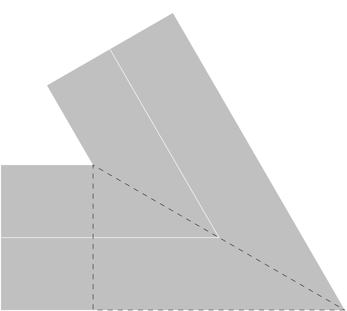
Miter Join
In Miter Join, the white lines represent the constructed line segments, and the gray area represents the results of stroking the path. In addition, we have overlaid a dashed right triangle. The height of this triangle is the line width of the stroked path. The hypotenuse of this triangle is called the miter length. The miter length is evidently proportional to the line width. If the segments meet with an angle of \(\theta\), then the relative miter length is \(1 / \sin(\theta / 2)\). [17]
| [17] | When two line segments meet, there is some ambiguity when we refer to the angle at which they meet. Restricting ourselves to angles that are fractions of a complete turn, we still must choose between the reflex angle and its explement. We refer to the reflex angle as the exterior angle, and we refer to its explement as the interior angle. Intuitively, this angle is interior to the triangle formed as the convex hull (or “fill”) of these two segments. In this context, we also use the term ‘angle’ as a synonymous with ‘interior angle’. |
The relative mitre length grows without bound as the two line segments become increasingly parallel.
For this reason, PostScript honors a limit on the relative miter length.
Whenever the relative miter length exceeds the miter limit,
PostScript automatically replaces a miter join with a bevel join.
The default limit is 10,
and the value can be set with the setmiterlimit_ operator.
Exercise
To construct Isoceles Triangle, we constructed a single path consisting of three joined line segments. How will our figure change if we construct the three segements as three separate paths, stroking each? (Assume the default butt line cap.)
Exercise
How will setting the miter limit to 1 affect our line joins?
Local Variables
It can be desirable to use variables in procedures. Although relying on stack manipulation is generally faster, variables can make our procedures easier to understand and maintain. As we know, any new variable definition will be in the current dictionary. It follows that we can limit the scope of a variable to the procedure in which it is defined only if we introduce a new current dictionary that exists only during the execution of the procedure.
Fortunately, this is very simple. The current dictionary is just the top dictionary on a separate dictionary stack. (For brevity, we will call this the dstack.) We can create a new dictionary with the dict operator, which takes a single integer argument (the initial capacity). We use the begin operator to move this dictionary from the ostack to the dstack, which makes it the current dictionary. Consider the following code.
1 dict
begin
/x 250 def
end
The first line creates a new dictionary with an
initial capacity for one key-value pair
and pushes it onto the ostack.
The begin operator pops the dictionary off the ostack
and pushes it on the dstack,
where it becomes the current dictionary.
Our variable definition adds an entry to the current dictionary.
The end operator pops the current dictionary off
the dictionary stack and discards it.
As a result, our definition of x is now discarded as well.
A Simple Arrow
The previous subsection explained miter joins. We now put these to good use by designing a simple arrow. We will do this by extending the current path with an arrow to the specified point, and then start a new subpath (with the moveto operator) at that point. We rely on a couple simplifications. Most importantly, we use the currentlinewidth when constructing the arrow. (This means that the arrow will not be accurate if we change the line width after constructing the arrow but before stroking it.) We also assume the use of mitre joins for stroking the path. (Otherwise, the arrowhead will not have a sharp tip and will fall slightly short of the new endpoint.) As a minor simplification, we assume a positive shaft length for the arrow. (We give a more thorough discussion of arrows in Arrows.)
/simpleArrowTo {12 dict begin
  /y exch def
  /x exch def
  currentpoint
  y sub neg /dy exch def                    %dy along arrow
  x sub neg /dx exch def                    %dx along arrow
  /alen dx dx mul dy dy mul add sqrt def    %total length of arrow
  /heading dy dx atan def                   %heading of arrow
  /theta 60 def                             %angle of arrowhead
  /turn 180 theta 2 div sub def             %turn angle of barb
  /width currentlinewidth def               %line width of arrow
  /blen 8 width mul def                     %barb length
  /mlen width theta 2 div sin div def       %miter length
  /slen alen mlen 2 div sub def             %shaft length
  slen heading fromPolar2D rlineto          %construct the shaft
  currentpoint                              %store pt A (end of shaft)
  blen heading turn add fromPolar2D rmoveto %move to end of one barb
  lineto                                    %construct one barb; consume pt A
  blen heading turn sub fromPolar2D rlineto %construct other barb
  x y moveto                                %move to tip of arrow
end}def
Our simpleArrowTo procedure makes unfettered use of local variables.
It also makes use of our previously defined fromPolar2D procedure.
The length and angle of the arrowhead have no theoretical justification
but are adequate in many circumstances.
The basic idea is to draw a line segment from the current point
to the new endpoint,
and then overlay an arrowhead at the endpoint.
If we were to do this naively,
we would do everything relative to the new endpoint.
But our discussion of mitre joins alerts us to an implication of doing so:
the tip of the arrow would extend past the new endpoint.
We therefore shift the arrowhead back by half of the mitre length,
and we similarly short the shaft of the arrow.
Arrays and Loops
We create an array by bracketing a sequence of objects. You can do any operations you wish as you create the array. For example,
[]                  %empty array
[ 1 pop ]           %empty array
[ 1 2 3 4 5 ]       %array of 5 integers
[ 1 2 add 3 4 mul ] %array of 2 integers
The left bracket just sets a mark, and the right bracket creates an array down to that mark, leaves that array on the ostack. More accurately, the item left on the stack is a reference to the array (which resides in `virtual memory`_).
Naturally you can retrieve objects from an array,
using the get operator and an array index.
Arrays use zero-based indexing:
the index of the first object in the array is 0.
For example, the following code fragment leaves 1 on the ostack.
[ 1 2 3] 0 get
Getting the first element of an array is common enough that we will create a named procedure for it. (This definition uses the bind operator, which we discussed in Bind.)
/head {0 get} bind def
We can also use the getinterval_ operator to extract any subinterval of the array. The getinterval_ operator consumes an array, an initial index, and a final index. It pushes on the ostack a new array, which contains the elements of the specified array interval. (The interval is specified as an initial index and a number of elements.)
Getting all but first element of an array is common enough that we will create a named procedure for it. In order to do so, we make use of the length operator, which returns the length of the array.
/tail {              % a0
  dup length 1 sub   % a0 len (len is a1's length)
  1 exch             % a0 1 len
  getinterval        % a1 (the tail of a0)
} bind def
Since the length operator consumes its operand,
we begin by duplicating the array on the ostack.
(This is very cheap; it just duplicates a reference to the array.)
We then find the length and subtract 1,
leaving the number of elements in the subarray.
We then push 1 on the stack and exchange that
with the number of elements,
giving us the interval specification we need.
Finally, we get that interval.
Arrays are mutable. We use the put operator to replace a single array element at a given index. Note that the put operator consumes three arguments from the ostack, but it does not push any. Consider the following lines of code.
1 1 5 iRange      %push array on ostack
dup               %push copy on ostack
0 99 put          %replace first element with 99 (consumes copy)
0 get             %get the first element of our "original" array
First we push an array on the stack.
(The object on the stack is actually a reference to our array.)
Then push a copy of that array on the stack.
(This is actually a copy of the reference.)
Next we change the copy.
Remember, the put operator consumes three operands,
so all that is left on the stack is our “original” array.
Finally, we use the get operator to retrieve the first
item of this array:
it is 99.
Arrays are mutable;
the put operator changed an element in our original array.
Arrays via Looping
Rather than enumerating the elements by hand, we usually want to create our arrays in some automated way. For this we can use looping constructs. The simplest looping operator is repeat. It requires two operands: a positive integer and a procedure. As a simple example, consider the following line of code:
[ 100 {0} repeat ]
First we push a mark on the stack,
signalling the begining of our array.
Then we push 100 on the stack;
this is how many times we will repeat the subsequent procedure.
Then we push a procedure on the stack,
which will be executed each repetition.
In this case, it simply pushes a 0 on the stack.
When the interpreter encounters repeat,
it consumes the top two objects on the ostack
and executes the procedure one hundred times.
This pushes 0 on the ostack one hundred times.
Finally, the bracket operator consumes all the operands down to the initial mark
and creates an array from the one hundred zeros.
This gives us a simple way to create any constant array.
The for loop is also useful for array creation.
It differs a bit from for loops in familiar imperative programming languages.
It takes four arguments:
three numbers to describe a numeric range,
and a procedure to apply to each value in that range.
The range is described by an initial value, an increment, and a limit value.
It also requires a procedure to execute at each iteration.
x dx xmax proc for ---
This description is slightly tricky: understand that each value in the range is pushed on the stack, and then the procedure is applied to it. For example, let us consider the effect of
[ 0 1 99 {}for ] %array of positive integers
Since the empty procedure is a no-op,
the range of values pushed on the ostack are not consumed.
This code fragment will therefore push onto the ostack
the nonnegative integers up to and including 99.
(Note that 99 is included; the limit is inclusive.)
This provides us with a very general approach to creating an integer range.
Creating an integer range is common enough that we will create a named procedure for it. Our procedure consumes three numbers (start, step, stop) that describe the range, and it returns an array containing the range. We retain the inclusive upper limit of the PostScript for operator.
/iRange {[ 4 1 roll {}for ]} def
We name the procedure iRange to emphasize that it
can include both endpoints.
We begin by pushing a mark on the ostack,
which will mark the left end of our new array.
We roll this below the range specification,
so that the mark is in the right place on the stack.
With three numbers at the top of the stack,
we are ready to make familiar use of the for operator.
Exercise
How will 0 0.1 1 {} for change the ostack, and why?
Exercise
Define a factorial function using a for loop.
This function should consume one nonnegative integer and return \(n!\).
Use stack manipulation rather than variables.
PostScript uses 32-bit integers. What is the largest factorial you can produce with integer calculations in PostScript?
Basic Array Operations
PostScript provides the forall operator
for iteration over arrays and dictionaries.
For now, we focus on iteration over arrays.
Used on arrays,
forall is essentially the foreach loop common in other languages.
Given an array and a procedure,
starting with the first item (whose index is 0),
an element is pushed on the ostack and the provided procedure applied to it.
For example, we can define a sum procedure for numercal arrays as follows.
/sum {0 exch {add} forall} bind def
This works by pushing 0 on the ostack and then swapping the top two items,
so that the array is back on top.
Next we push on the top of the ostack the anonymous procedure {add}.
The forall operator consumes the top two operand (i.e., the array and the procedure)
and then iterates over the array items,
pushing each item on the ostack and then executing the procedure.
We can define a map procedure for numerical arrays as follows.
% [num] (num -> num) *map* [num]
/map {
  [           %push mark on stack
  3 1 roll    %move mark before array
  forall      %execute function for each array item
  ]           %create array from new items on stack
} bind def
Developing a zip procedure gives us a change to
explore our understanding of arrays.
% [num] (num -> num) *map* [num]
/map {
  [           %push mark on stack
  3 1 roll    %move mark before array
  forall      %execute function for each array item
  ]           %create array from new items on stack
} bind def
With map and zip in hand,
we can readily implement basic elementwise operations on arrays.
% [num] (num -> num) *map* [num]
/map {
  [           %push mark on stack
  3 1 roll    %move mark before array
  forall      %execute function for each array item
  ]           %create array from new items on stack
} bind def
Arrays as Line Descriptions
In this booklet, we will use arrays of numbers to describe points. For example, we will use [0 0] to describe the origin. We can use an array of points to descibe a line. For example, [[0 0] [1 1]] describes a line from the origin to the point [1 1]. However we want to something different with the first point (move to it) than with the others (add a line sement to the path). In recogntion of this, we will create an deconstruction operator, which consumes an array and returns its tail and its head.
/uncons {     %arr
  dup         %arr arr
  tail exch   %tail arr
  head        %tail head
} bind def
Now if we have an array of points,
we can apply our uncons procedure to get the first point
on the top of the stack and an array of the others right below it.
But PostScript drawing operators work with numbers on the ostack,
not with arrays.
In order to construct a line with our familiar PostScript operators,
we are going to have to get our hands on the individual coordinates.
In order to push the items of an array onto the ostack,
we use the aload operator.
The aload operator pushes all the array items individually on the ostack.
The aload operator consumes an array and pushes all its elements onto the stack,
but then it also pushes the array itself back onto the stack.
We just want the elements,
so we use the pop operator to discard the array on the top of the stack.
Now we are ready to construct a line from a list of points.
/polyLine {
  uncons               %tail head
  aload pop moveto     %tail
    {aload pop lineto} %tail proc
  forall               % --
} bind def
Exercise
Define three (non-colinear) points,
using arrays.
Make an array of these points.
Use our polyLine procedure
to construct a triangle using this array of points.
Stroke your triangle with a black line of width 2.
Define a midpoint procedure that
consumes two points and returns a point.
Use your midpoint procedure to
draw the three medians of your triangle.
Stroke your triangle medians with a gray line of width 1.
You should end up with something along the lines of
Triangle with Medians.
Hint: use the closepath operator.
Triangle with Medians
Project: Circle Points
This project is oriented more toward programming than toward drawing.
We will produce a list of evenly spaced points drawn from the unit circle.
There is a single integer argument, n,
the number of points.
The points are structured so that if used to draw a polygon,
the polygon will have a horizontal base.
% n circlePoints [pt]
/circlePoints {3 dict begin /n exch def
  /angle 360 n div def
  /angle2 angle 2 div def
  [
  0 1 n 1 sub {[ exch angle mul angle2 add 270 add dup cos exch sin ]}for
  ]
end} def
The circlePoints procedure is a fun demonstration of some
basic computations in PostScript.
However, it is not yet very useful for drawing actual polygons.
We could handle this in a few different ways, and we will.
For the moment, let us consider simple procedures to scale
up these points and translate them.
% [pt] s *scalePoints* [pt]
/scalePoints {1 dict begin /s exch def
  {s exch s:mul} map
}def

% [pt] pt *translatePoints* [pt]
/translatePoints {1 dict begin /t exch def
  {t a:add} map
end}def
Now we are ready to construct regular polygons of any size wherever we want.
% x y r n centeredRegularPolygon ---
/centeredRegularPolygon {
  circlePoints exch scalePoints
  [ 4 -2 roll ] translatePoints
  polyLine closepath
}def
E.g., to produce a dodecagon centered on the page, we could do the following.
306 396 216 12 centeredRegularPolygon
Transformations
User Space
Our first PostScript examples illustrate the very natural coordinate system PostScript provides for describing positions on the page. We begin with a standard Cartesian coordinate system, with the origin at the bottom left corner of the page. This is the coordinate system we initially encounter---the default user space. The default user space is device-indpendent in the following sense: we do not need to know anything about how the output device characterizes its drawing space. We just attend to the user space; we do not need to understand the device space. This is very convenient: we can write one PostScript program and produce the output on many different devices.
Of course we cannot always hope for complete ignorance of the device. For example, a printer may handle only certain paper sizes, and it may not be able to print at the very edge of the page. And naturally, a low-resolution device may not be able to render all the high-resolution details of a drawing. Still, PostScript allows us to be as agnostic as possible about the device on which a drawing will be rendered.
Up to now we have mostly been drawing in the default user space. However, we are free to change the current user space with transformation operators. These change the coordinate system in which the programmer is drawing. We can translate the origin or rotate the orientation of our coordinate system. We can also scale the unit size. Such transformations affect subsequent path construction and painting, but they do not affect any path construction or painting that we have completed. For example, transformations do not move the location on the page of the current point or the current path. In this section we will see how this can be useful.
This section discusses three operators for simple coordinate system transformations. (For additional detail see [adobe-1985-pltc] [ch.6].) These are translate, scale, and rotate. These operators effectively allow us to move our axes for drawing around on the page: we can shift them horizontally or vertically, we can “stretch” or shrink them (so that the axes are not moved but their units are changed), or we can rotate them around the current origin. We can invoke these operators even in the midst path construction, and they will only affect the construction subsequent to the invocation. This section discusses the effects of these transformations and offers a simple but useful illustration.
- Translate
- The translate operator changes the location of the user space origin. Consider the location on the page associated with the coordinates \((dx,dy)\) in the current user space. The instructions dx dy translate will move the origin \((0,0)\) to that location. Each location on the page has its coordinates transformed in this fashion. The new coordinate system constitutes the new user space. The origin can be translated along both axes (i.e., both horizontally and vertically relative to the current user space). The two operands specify the x-axis translation the y-axis translation. For example, a location on the page that had coordinates \((x0,y0)\) will, subsequent to the translation, have coordinates (x0+dx, y0+dy).
- Rotate
- We can also rotate the coordinate axes of the user space.
Use the command theta rotate
to rotate the axes
thetadegrees counterclockwise. Every location on the page has its coordinates changed appropriately to produce the new user space. This does not move the origin or change the scale. - Scale
- The scale operator allows us to change the units
on the coordinate axes
without affecting the origin or the orientation of the axes.
The command sx sy scale imposes a
“horizontal” scale factor of
sxand a “vertical” scale factor ofsy. For example, the location on the page that had coordinates \((x0,y0)\) will, subsequent to the scale operation, have coordinates \((x0/sx, y0/sy)\).
Clearly order matters when using scale and translate. If scale comes first, the scaled units will be used in translating the origin of the user coordinate system.
Project: Equilateral Triangle
In Isoceles Triangle, we drew an isoceles triangle. In the process, we gained the tools to draw any figure consisting of straight line segments as long as we can specify the endpoints (or relative endpoints) of each segment. Sometimes such specification can require avoidable effort, however. For example, instead of an isoceles triangle we may wish to draw an equilateral triangle. The equilateral triangle is a common representation of the two dimensional simplex, so it shows up in a diversity of contexts. [18]
| [18] | Economic examples include the illustration of sectoral shares, the representation of strategy sets, illustration of the stability properties of tatonnement, representation of the allocation probabilities for an indivisible good, game theoretic proofs, and proofs related to social choice, public choice, and mechanism design. For randomly chosen illustrative examples from textbooks and journal articles see [carter-2001-mit] [ch.1], [hildenbrand.kirman-1988-elsevier] [section 6.5], [karni.safra-2002-e], [laffont-1988-mit] [ch.2], [moulin-2000-e] [Appendix], or [stengel.elzen.talman-2002-e]. |
Once we draw one side of an equilateral triangle, we must face the question of how to draw the second side. The brute force way is to trigonometrically compute the location of the second vertex and then draw a line segment to that point. [19] A simpler solution is to exploit our ability to characterize any triangle by a side, an angle, and a second side. In PostScript, after drawing the first side, we can translate the origin to the endpoint of the first line segment, rotate clockwise around the new origin by 120 degrees, and then draw the second side exactly like the first one. We will write the code to do this so that it makes use of our three transformation operators.
| [19] | Since PostScript includes sin and cos operators this is actually a reasonable approach. For example, if we begin by drawing a side of length 10 we could proceed to draw a second side as currentpoint 120 sin 10 mul add exch 120 cos 10 mul add exch lineto. |
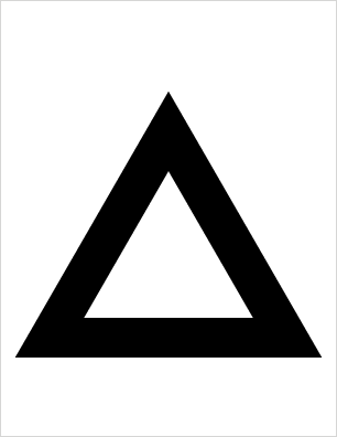
Equilateral Triangle: Stroked
%!
72 72 scale          %set units to inches
1.25 2.5 translate   %translate origin
0 0 moveto           %moveto origin
6 0 lineto           %construct first 6" line segment
6 0 translate        %translate origin to current point
120 rotate           %rotate axes 120 degrees counterclockwise
6 0 lineto           %construct second line segment
closepath            %construct final line segment
stroke               %paint the constructed triangle
showpage             %view the result
Fist consider the result of stroking the constructed path. You may be surprised by the display in Equilateral Triangle: Stroked. Specifically, why is the line width of the stroked triangle so large? The reason is that the default line width is one unit (along each axis), but we used the scale operator to scale the unit to one inch. (The drawing displays as it would on a sheet of letter paper, the boundary of which appears as a light gray outline.) So the line width used for stroking is a full inch. (We will learn how to deal with this when we discuss the graphics state.)
Grayscale
In addition to stroking the resulting path in black, we will fill it with gray. This will introduce notions of color and filling. We have seen that in PostScript path construction is distinct from painting (i.e., stroking or filling). Stroking and filling can be done with any color, including any desired shade of gray. As an analogy, we might think of setting the color as choosing your ink. All colors are opaque, including white, so newly applied “ink” completely covers anything beneath it. [20]
| [20] | The PostScript graphics model does not support transparency.
The PDF graphics model extends the PostScript model to support transparency.
The pdfmark extension to PostScript allows a representation of transparency
that is not usable by PostScript interpreters,
but only by PDF interpreters (after the PostScript has been “distilled” to PDF).
http://www.adobe.com/content/dam/Adobe/en/devnet/acrobat/pdfs/pdfmark_reference.pdf
(The pdfmark extension to PostScript allows the inclusion of
several other PDF features as well.)
In PostScript, transparency can be emulated by rasterization. |
To pick a shade of gray we use the setgray operator, which takes a single numerical operand between zero and one. As an analogy, we might say the operand signifies the proportion of white ink, where the remainder is black ink. So 0 setgray selects “black ink” for all subsequent markings on the page, while 1 setgray selects “white ink”. [21] Numbers between 0 and 1 select various shades of gray.
| [21] | Since our first drawings were all in black, it should be clear that this is the default color for a PostScript interpreter. The initial color space is DeviceGray. Alternative color spaces are DeviceRGB and DeviceCMYK. A device color space specifies the colors that the output device should produce. A discussion of color spaces is beyond the scope of this booklet, but we will nevertheless make use of color in our drawings. |
Exercise
Right before stroke in the above code,
add the line of code 0.5 setgray fill.
Display the result.
You will see our previous triangle, but now gray in color.
Next, change stroke to fill, and display the result.
You will see a filled gray triangle.
Graphics State
A bit like the man who discovered that he had been speaking prose all his life,
we now acknowledge that we have been manipulating the graphics state all along.
The current graphics state holds such things as the current path,
the current line width, the current color, the current clipping path,
the current font, and the current user space.
([adobe-1999-plrm3] [section 4.2] offers a full discussion.)
Since the current color is part of the graphics state,
0.5 setgray changes the graphics state
to specify a medium gray for any painting operations.
We can choose fill or stroke as our painting operation.
Often it is useful to temporarily save at least part of the graphics state for reuse.
Most of the time we do this with the gsave and grestore operators. [22]
A common application arises when
we wish to both stroke and fill the same path.
Both stroke and fill perform an implicit newpath operation and thereby destroy the current path.
We could of course explicitly construct the path twice,
once for stroking and once for filling.
A second approach proves more convenient.
Since the current path is part of the graphics state,
we can save the graphics state with the gsave operator before stroking the path.
After stroking it,
we can restore the path with the grestore operator,
so that it is available for filling.
Concretely, in the above code,
replace stroke with gsave stroke grestore 1.0 setgray fill.
| [22] | That is, we use the gsave operator to push the entire current graphics state onto a special stack, called the graphics state stack. We use the grestore operator to pop the saved graphics state from the graphics state stack when we need it again later. |
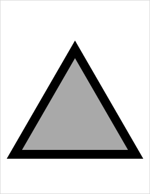
Equilateral Triangle
%!
72 72 scale          %set units to inches
1.25 2.5 translate   %translate origin
0 0 moveto           %moveto origin
6 0 lineto           %construct first 6" line segment
6 0 translate        %translate origin to current point
120 rotate           %rotate axes 120 degrees counterclockwise
6 0 lineto           %construct second line segment
closepath            %construct final line segment
gsave                %save the graphics state
stroke               %paint the constructed triangle
grestore             %restore the graphics state
0.6 setgray          %change color to medium gray
fill                 %fill the path
showpage             %view the result
Program Details
Line by Line
We will now consider this PostScript program line by line. As always the first line of our program is a special comment, which declares it to be a PostScript program, and the last line is the showpage operator.
The second line scales the units so that along each axis one unit is now 72 points (i.e., one inch). We then use the translate operator to move the origin of user space to the first vertex of our triangle. (The position of the first vertex is arbitrary: for this example we chose to center the triangle horizontally on a sheet of letter paper and to construct the triangle one inch above the bottom of this sheet.) Now we are ready to construct the path describing our equilateral triangle. We begin path construction by moving to the (new) origin, and we then construct our first 6 inch line segment along the bottom of our triangle. Next we move the origin of user space to the second vertex, in preparation for a rotation of user space. We rotate our axes by 120 degrees, which implies that we can construct the second side of our triangle simply by moving right along the “x-axis", exactly as we constructed the first side. The final line segment is constructed for us automatically when we use the closepath operator. That completes the path construction for our triangle.
This is a very simple way to construct a perfect equilateral triangle: much simpler than in many point and click drawing programs. (Furthermore, by analogy, we can with equal ease construct a regular polygon with any number of sides.) Once we have constructed our path, we are ready to stroke or fill it. This time we will do both, but this creates a small problem. The fill and stroke operators each finish with an implicit newpath command, which destroys the path we have constructed. We could stroke the path and then reconstruct it from scratch for our fill operation, but as we saw in the section on Color_ there is a better way. The gsave operator allows us to save a copy of our constructed path, and the grestore command allows us to retrieve this saved copy. So before we stroke our constructed path with the default color (black), we save the current path with the gsave operator. After our stroke operation, we use the grestore operator to restore that path, which we can then fill. Before we fill it, we change the current color to gray. The showpage operator will then show us figure Equilateral Triangle.
PyX: Equilateral Triangle Project
After setting the defaultunit to 1 inch for our drawing, we construct our triangle in three steps. As in the PostScript version, we begin by constructing the first side as a 6 inch long horizontal line segment. To construct the second side, however, we have to consider a crucial difference in the PyX transformation concept. Whereas in PostScript we transform the userspace and then construct our paths in the transformed space, in PyX we effectively construct our paths in a fixed user space but we can then transform them.
So we cannot rotate the user space as we did in PostScript.
Instead, we take the point \((6,0)\)
and rotate it around the origing by 120 degrees.
This produces the relative movement needed to reach
the next endpoint for our path construction.
The statement x,y = trafo.rotate(120).apply(6,0)
produces a rotation transformation and applies it to the point
\((6,0)\),
producing the coordinates of the rotated point.
These are the relative coordinates of the point we are seeking.
The key is to see that these coordinates provide the relative
movements we wish to make from the point \((6,0)\).
So we can construct our second line segment as rlineto(x,y).
Constructing the third side is as simple as in PostScript:
we just close the path to complete our triangle.
Unlike PostScript,
PyX uses the concept of a canvas.
We do our drawing on a canvas.
(Canvases can also be transformed.)
We now need to create a canvas cvs
and stroke this triangle on the canvas,
but first we decide on some style attributes for the triangle.
To match our previous PostScript drawing,
we set the color to a medium gray,
set the line width to 1 inch,
and translate the triangle 1.25 inches horizontally and 1 inch vertically.
(Again, note the difference in the approach to transformation:
we do not transform the user space, but rather we transform our constructed path.)
Finally we write our PostScript file using the
writePSfile method of our canvas. [23]
| [23] | You need to be careful with the writeEPSfile method of the
canvas, which as of version 0.10 does not always compute a
useful bounding box.
This code serves as a good test case: using writeEPSfile,
the bounding box for this figure cut off the corners of the triangle.
(The writeEPSfile method takes a bboxenlarge parameter,
which can be adjusted to deal with this problem.
You can also use Ghostscript to do the calculation:
gs -dNOPAUSE -q -dBATCH -sDEVICE=bbox -f myfile.ps.) |
For this particular drawing, PyX's caclulation of the bounding box is an issue. The bounding box computed by PyX will always include the paths we construct, but because we have set a very large line width, the “miter” produced at the corners when we stroke the patch extends beyond the bounding box. This will not be a problem if our drawing contains other items beyond these miters. Here we set our own bounding box. Alternatively, we can enlarge PyX’s bounding box.
from pyx import path, trafo
pyx.unit.set(defaultunit='inch')
triangle = path.path(path.moveto(0,0), path.rlineto(6,0))
#find the triangle apex as a relative location
x,y = pyx.trafo.rotate(120).apply(6,0)
triangle.extend([path.rlineto(x,y),path.closepath()])
#set the color, line width, and transformation of the whole path
strokeStyle = pyx.style.linewidth(1), trafo.translate(1.25,1)
fillStyle = pyx.color.gray(0.5), trafo.translate(1.25,1)
#we need a canvas to draw on
cvs.stroke(triangle, attrs=strokeStyle)
cvs.fill(triangle, attrs=fillStyle)
TikZ: Equilateral Triangle Project
For this particular drawing, TikZ’s caclulation of the bounding box is an issue. The bounding box computed by TikZ will always include the paths we construct, but because we have set a very large line width, the “miter” produced at the corners when we stroke the patch extends beyond the bounding box. This will not be a problem if our drawing contains other items beyond these miters. Here we set our own bounding box to the size of a full (letter size) page.
\begin{tikzpicture}[x=1in,y=1in]
\path[use as bounding box] (0,0) rectangle (8.5,11);
\path[shift={(1.25,2.25)},
      line width=1in,
      draw,
      postaction={fill=gray}
      ]
      (0,0)  -- ++(6,0) -- ([turn]120:6) -- cycle;
\end{tikzpicture}
HTML Canvas: Equilateral Triangle Project
When implementing Project 1,
we learned that CanvasRenderingContext2D
inverts the y-axis coordinates (relative to PostScript).
However, each CanvasRenderingContext2D object has a current transformation matrix,
initialized to the identity transform.
This means that CanvasRenderingContext2D supports familiar userspace transformations.
If we prefer to work with a more familiar representation of the Cartesian plane,
we can just translate the origin to the bottom left and then
scale the \(y\) coordinates by \(-1\).
From now on,
our code examples assume this transformation.
ctx.scale(72,72);
ctx.translate(1.25,2.5);
ctx.beginPath();
ctx.moveTo(0,0);
ctx.lineTo(6,0);
ctx.translate(6,0);
ctx.rotate(120*Math.PI/180);
ctx.lineTo(6,0);
ctx.closePath();
ctx.lineWidth = 1;
ctx.stroke();
After the initial boilerplate, constructing this drawing on an HTML canvas closely resembles the corresponding PostScript code. Here are some simple correspondences.
| PostScript | CanvasRenderingContext2D |
|---|---|
| 0 1 translate | translate(0,1) |
| 3 4 scale | scale(3,4) |
| 5 rotate | rotate(5*Math.PI/180) |
| 0.0 setgray | strokeStyle = 'Black' |
| 0.6 setgray | fillStyle = 'Gray' |
fill |
fill() |
The immediately noticeable difference is that
we must now measure the angle of rotation in radians,
whereas PostScript measures it in degrees.
However, the color model is also vary different.
We can separately specify a fillStyle and a strokeStyle,
and we set these to a string value.
(We will discuss this further in Colors.)
Finally,
the path we have constructed
is not discarded when we stroke it.
So although we stroke our path without first saving the graphics state,
we can still subsequently fill it.
Mathematica: Equilateral Triangle Project
Mathematica provids an AnglePath command
to implement turtle graphics:
angular relative movements in along a path.
We can provide AnglePath with an initial point,
corresponding to a PostScript moveto,
and a list of steps.
Here we specify each step as a length and a relative angle.
Since Mathematica commands expect angles in radians,
for convenience with PostScript,
we defined a deg2rad constant.
deg2rad = \[Pi]/180
relpts = AnglePath[{0, 0}, {{6, 0}, {6, 120 deg2rad}}]
Mathematica does not support the concept of userspace transformations.
Our first approach will be to use vector algebra to produce
an affine transformation of relpts.
We then use Line to produce the triangle sides,
and JoinedCurve and FilledCurve to stroke and fill the triangle.
pth = Line[72*({5/4, 5/2} + # & /@ relpts)]
stroked = JoinedCurve[pth, CurveClosed -> True]
filled = FilledCurve[pth]
g1 = Graphics[{Black, Thickness[72/612], stroked, GrayLevel[0.6], filled},
  PlotRange -> {{0, 612}, {0, 792}},
  ImageSize -> {612, 792}
]
Although Mathematica does not support the concept of userspace transformations,
it does support transformations of graphics objects.
So we can alternatively construct our equilateral triangle as follows.
We will use Mathematica’s Scale and Translate commands
to produce a transform function that implements our scaling
and translation.
There is one new detail:
by default, Scale does its scaling relative to the center of the
bounding box of the graphic.
We do not want that.
Fortunately, Scale accepts a second argument,
where we can specify that we want scaling to be relative to the origin.
(That is, we want the origin in our graphic to remain fixed.)
Apply our new transform function to a JoinedCurve and a FilledCurve,
each based on the relative path we first described using AnglePath.
Then use this to produce our overall graphic as before.
relpth = Line[relpts]
transform = Scale[Translate[#, {5/4, 5/2}], {72, 72}, {0, 0}] &
stroked = transform@JoinedCurve[relpth, CurveClosed -> True]
filled = transform@FilledCurve[relpth]
Finnally, we illustrate how to use GeometricTransformation to produce a transformation function,
which we name transform02.
We use a composition of a ScalingTransform and a TranslationTransform.
transform02 = GeometricTransformation[#,
  ScalingTransform[{72, 72}]@*TranslationTransform[{5/4, 5/2}]] &
Project: Pythagorean Theorem
Our next project will make use of some of our new PostScript programming skills. [isaacs-1975-mathmag] presents a classic “proof without words” of the Pythagorean theorem, illustrated here by Pythagorean Theorem.
Pythagorean Theorem
Since all of the triangles are congruent, the area of the dark square in the first subfigure evidentally equals the combined areas of the dark squares in the second subfigure. In attacking this project, we will use of coordinate system transformations. Additionally, we will need to some control over color and over the graphics state. color, and the graphics state.
/a 60 def        %triangle base
/b 120 def       %triangle height
/ab a b add def  %base + height

% x y s *square* --
% construct square at coordinates (x,y) with side length s
/square {1 dict begin /s exch def
  moveto s 0 rlineto 0 s rlineto s neg 0 rlineto closepath
end} def

% x y base height *rtTriangle* --
% construct upright right triangle at (x,y) with side lengths (base,height)
/uprightTriangle {2 dict begin [/height /base] {exch def}forall
  moveto base 0 rlineto base neg height rlineto closepath
end} def

%stroke and fill styles for constructed figures
/styleTriangle {gsave 0.9 setgray fill grestore 0 setgray stroke} def
/styleSquare {gsave 0.6 setgray fill grestore 0 setgray stroke} def
Now consider the first subfigure.
0 0 ab square styleSquare
4 {0 0 a b uprightTriangle ab 0 translate 90 rotate} repeat
styleTriangle
Now consider the second subfigure.
0 0 ab square styleSquare
0 0 a b uprightTriangle ab b translate 90 rotate
0 0 a b uprightTriangle 0 b translate 90 rotate
0 0 a b uprightTriangle 0 a neg translate 90 rotate
0 0 a b uprightTriangle
styleTriangle
PyX: Pythagorean Theorem Project
Recall that transforming a path in PyX is equivalent to producing a linear transformation of every point in the path. Whereas in PostScript we transform the userspace and then construct our paths in the transformed space,
import pyx
from pyx import trafo, deco, style, color
from pyx.canvas import canvas
from pyx.path import path, moveto, rlineto, rmoveto, closepath
pyx.unit.set(defaultunit='pt')

#BEGIN definitions
a = 72
b = 144
ab = a + b
bigsquare = path(moveto(0,0), rlineto(ab,0), rlineto(0,ab), rlineto(-ab,0), closepath())
triangle = path(moveto(0,0), rlineto(a,0), rlineto(0,b), closepath())
triangle_style = [color.gray(0), deco.filled([color.gray(0.9)]) ]
square_style = [color.gray(0), deco.filled([color.gray(0.6)]) ]
#END definitions

#set defaults
cvs = canvas(attrs=[style.linejoin.bevel, pyx.style.linewidth(1)])

#BEGIN subfigure1
cvs.stroke( bigsquare, square_style)
triangles = [ triangle ]
for i in range(3):
  newpath = triangles[-1].transformed(trafo.rotate(90).translated(a,b))
  triangles.append(newpath)
cvs.stroke( sum(triangles,path()).transformed(trafo.translate(b,0))  , triangle_style)
#END subfigure1

#BEGIN subfigure2
figoffset = trafo.translate(234,0)
cvs.stroke( bigsquare.transformed(figoffset), square_style)
t2 = triangle + triangle.transformed(trafo.rotate(180).translated(a,b))
t4 = t2 + t2.transformed(trafo.rotate(90).translated(ab,b))
cvs.stroke( t4.transformed(figoffset), triangle_style)
#END subfigure2


cvs.writeEPSfile('d:/temp/temp.eps')
HTML Canvas: Pythagorean Theorem Project
There is only one CanvasRenderingContext2D object per canvas.
Calling getContext with the 2d argument a second time returns the same object.
This means we cannot build up paths in two separate contexts
(for a single canvas).
The transformations must be performed in reverse order. For instance, if a scale transformation that doubles the width is applied to the canvas, followed by a rotation transformation that rotates drawing operations by a quarter turn, and a rectangle twice as wide as it is tall is then drawn on the canvas, the actual result will be a square.
| PostScript | CanvasRenderingContext2D |
|---|---|
gsave |
save |
grestore |
restore |
| 0 1 translate | translate(0,1) |
| 3 4 scale | scale(3,4) |
| 5 rotate | rotate(5*Math.PI/180) |
| 0.0 setgray | strokeStyle = 'Black' |
| 0.6 setgray | fillStyle = 'Gray' |
fill |
fill() |
Recall that PostScript maintains a `graphics-state stack`_,
which we nickname the gstack_.
A CanvasRenderingContext2D maintains a similar stack of drawing states that comprises:
- current transformation matrix.
- current clipping region.
- current attributes values (strokeStyle, fillStyle, globalAlpha, lineWidth, lineCap, lineJoin, miterLimit, shadowOffsetX, shadowOffsetY, shadowBlur, shadowColor, globalCompositeOperation, font, textAlign, textBaseline)
This is often called the drawing-state stack,
but to emphasize the comparison to PostScript,
we will call it the canvas gstack_.
A CanvasRenderingContext2D has save and restore methods
to push to and pop from the gstack_.
We begin by defining some model variables, including our drawing functions and styling function.
var a=60, b=120, ab=a+b;
var drawSquare = function(c, x, y, s) {
  c.moveTo(x,y); c.lineTo(x+s,y); c.lineTo(x+s,y+s); c.lineTo(x,y+s);
  c.closePath();
};
var drawTriangle = function(c, x, y, b, h) {
  c.moveTo(x,y); c.lineTo(x+b,y); c.lineTo(x,y+h);
  c.closePath();
};
var styleSquare = function(c) {
  c.fillStyle = 'DarkGray'; c.strokeStyle = 'Black';
};
var styleTriangle = function(c) {
  c.fillStyle = 'LightGray'; c.strokeStyle = 'Black';
};
Next, we draw the first subfigure.
Once again, our approach is to emphasize parallels to our PostScript implementation.
Note that we use several transformations in this drawing,
so we wrap it in a save and restore.
ctx.save();
//draw the large square
ctx.beginPath();
drawSquare(ctx, 0, 0, ab);
styleSquare(ctx); ctx.fill(); ctx.stroke();
//draw the four triangles
ctx.beginPath();
let i=4; while(i--) {
  drawTriangle(ctx, 0, 0, a, b);
  ctx.translate(ab,0);
  ctx.rotate(Math.PI/2);
}
styleTriangle(ctx); ctx.fill(); ctx.stroke();
ctx.restore();
Finally, after an appropriate translation to separate the two figures, we are ready to draw the second subfigure.
ctx.beginPath();
drawSquare(ctx, 0, 0, ab);
styleSquare(ctx); ctx.fill(); ctx.stroke();
ctx.beginPath(); //draw four triangles
drawTriangle(ctx, 0, 0, a, b); ctx.translate(ab, b); ctx.rotate(Math.PI/2);
drawTriangle(ctx, 0, 0, a, b); ctx.translate(0, b);  ctx.rotate(Math.PI/2);
drawTriangle(ctx, 0, 0, a, b); ctx.translate(0, -a); ctx.rotate(Math.PI/2);
drawTriangle(ctx, 0, 0, a, b);
styleTriangle(ctx); ctx.fill(); ctx.stroke();
Mathematica: Pythagorean Theorem Project
As usual, our approach will be structured to promote
comparison with the PostScript code.
So we make use of our deg2rad constant introduced
in the previous project.
Additionally, we freely introduce global variables
(a, b, and ab).
We will again use the Translate command,
but first we make use of the Rotate command.
The rotate command rotates a graphic object around
a specified point.
We will produce a base triangle at the origin,
and then use Rotate to produce rotations around the origin.
Once we have our rotated triangles,
we will place them appropriately by translating them.
Keep in mind that in Mathematica we rotate and translate graphic objects,
whereas in PostScript we rotate and translate the userspace
(relative to the device space).
a = 60; b = 120; ab = a + b;
pathSquare = Function[{x, y, s},
  Line@Accumulate[{{x, y}, {s, 0}, {0, s}, {-s, 0}}]];
pathTriangle = Function[{x, y, b, h},
  Line@Accumulate[{{x, y}, {b, 0}, {-b, h}}]];
styleSquare = Sequence[EdgeForm[{Thickness[1/ab], Black}],
   FaceForm[GrayLevel[0.6]]];
styleTriangle = Sequence[EdgeForm[{Thickness[1/ab], Black}],
   FaceForm[GrayLevel[0.9]]];
filledSquare = FilledCurve[pathSquare[0, 0, ab]];
(* base triangle, to rotate and translate *)
t1 = FilledCurve[ pathTriangle[0, 0, a, b]];
(* produce all the rotations *)
{t2, t3, t4} = Rotate[t1, #, {0, 0}] & /@ ({90, 180, 270} deg2rad);
We are now ready to produce our first subfigure. We just need to appropriately translate each of our rotated triangles, and put everything together in a single graphic.
t2a = Translate[t2, {ab, 0}];
t3a = Translate[t3, {ab, ab}];
t4a = Translate[t4, {0, ab}];
g1 = Graphics[{styleSquare, filledSquare, styleTriangle, t1, t2a, t3a, t4a}]
The second subfigure is constructed from the same objects, except that we need different translations.
t2b = Translate[t2, {ab, b}];
t3b = Translate[t3, {a, b}];
t4b = Translate[t4, {a, ab}];
g2 = Graphics[{styleSquare, filledSquare, styleTriangle, t1, t2b, t3b, t4b}]
After constructing our two subfigures,
we can combine them with the GraphicsRow command.
GraphicsRow[{g1, g2}]
Dots
Zero Is Not Zero
For drawing, zero has a special meaning. A line width of zero means the thinnest line the rendering device is capable of drawing. A line length of zero means a zero length line, but it still includes other features. Specifically, it includes the line cap, which determines what happens at the end of the line. There are three possible values.
| linecap | meaning |
|---|---|
| 0 | butt cap (no projection) |
| 1 | round cap (half circle extension) |
| 2 | square cap (half square extension) |
This means we can create circles of a given radius by setting the line width to twice that radius and drawing a zero-length line. One might think that similarly we could create circles of a given radius by setting the line width to the side of the square and drawing a zero-length line. However this is not true, as the orientation of the resulting square would be unknown.
Circles
We can draw circles with the arc operator, which constructs all or part of a circle. The arc operator has five operands: the x and y coordinates of the center of the circle, the radius of the circle, the initial angle (at which to start constructing the arc), and the terminal angle. The angles are measured in degrees counterclockwise from the positive x axis. [24] (The arcn operator works the same way, except that it constructs the arc is clockwise.) So, for example, 306 396 10 0 360 arc will construct a full circle with center at \((306,396)\) and radius of 10 points, whereas 306 396 10 0 90 arc will construct only the first quarter of that circle.
| [24] | Changes to the user space can change the location, orientation, and scale of this axis, of course. |
Underneath, a circle is an approximation to a circular arc that is constructed from cubic Bézier segments [adobe-1999-plrm3] [p.530]. For the most part, we will not care about this detail, since this approximation is extremely accurate. Nevertheless it is a good idea to use the closepath operator on a 360 degree arc to account for approximation in the “perpendicular" extension for the line width at the endpoints of the arc. For example, a full circle drawn with a thick line width will display a “notch” unless the circular path is closed with the closepath operator.
We can use the arc operator even when no current point is defined. However, if the current point is defined, the arc operator additionally constructs a line segment from the current point to the beginning of the arc.
Storing Values for Later Use
Up to now, we have been placing operands on the stack when we are ready to use them. But we can push objects on the stack for later use as well. In our next project we will illustrate this by storing the current point several times during path construction. (We use the currentpoint operator to push the current point on the stack, as two numbers.) After that constructing the path, we will then retrieve these stored values for further use. It is common in PostScript drawing to store values for later use by pushing them on the stack.
Using the stack in this way is fast and cheap. A disadvantage to storing values on the stack for later use is that one must keep track of what is on the stack and where. Therefore we often store a value for later use by assigning it to a variable. The PostScript syntax for this is a bit unusual. We push a literal name on the stack by prepending a slash. Then we push a value on the stack. Then we use the def operator to associate the value with the name. (See Variables and Named Procedures for details.) For example,
/x 10 def %assign value 10 to variable `x`
Project 3
The next project exercises our understanding of circles in PostScript by producing the Circumscribed Circles. We will approach this as follows: draw the triangle, then the small circles, and finally the large circle. We will specify that the small circles have a radius of 1 inch (72 points), and that the figure is centered on the (letter-sized) page.
Circumscribed Circles
The figure is centered on the page. So our first task is to draw an equilateral triangle centered on a point. We will do this by starting at that point and then moving to the top of the triangle. Recall that the hypotenuse and long leg of a 30,60,90 triangle have length (relative to the short leg) of \(2\) and \(\sqrt{3}\). Since the triangle we want to draw is equilateral with a base of 2, the top is \(2/\sqrt{3}\) inches above the centroid. This also implies that the diameter of the large circle is \(1+2/\sqrt{3}\) inches.
306 396 translate              %move origin to center of page
/tht 3 sqrt 72 mul def         %triangle height
/tht23 tht 2 mul 3 div def     %2/3 of triangle height
0 tht23 moveto                 %start at top of triangle
currentpoint                   %store 1st circle location
-72 tht neg rlineto            %construct 1st side
currentpoint                   %store 2nd circle location
144 0 rlineto                  %construct 2nd side
currentpoint                   %store 3rd circle location
closepath                      %construct 3rd side
stroke                         %stroke the triangle

72 0 360 arc closepath stroke  %stroke 3rd circle
72 0 360 arc closepath stroke  %stroke 2nd circle
72 0 360 arc closepath stroke  %stroke 1st circle
%finally, stroke the big circle
0 0 72 tht23 add 0 360 arc closepath stroke
Project 3 in TikZ
In a (LaTeX) TikZ drawing,
simple constants can be assigned with \newcommand,
but we use pgfmathsetmacro
when our definition includes some computations.
Note that names must use alphabetic characters only.
We use (x,y)coordinate(myvar) to
association the coordinate \((x,y)\) with (myvar).
\begin{tikzpicture}[x=1bp,y=1bp,shift={(306,396)}]
\pgfmathsetmacro{\tht}{72 * sqrt 3}
\pgfmathsetmacro{\thttt}{\tht * 2 / 3}
\path[draw,line width=1]
  (0,\thttt)coordinate(p1)
  -- ++(-72,-\tht)coordinate(p2)
  -- ++(144,0)coordinate(p3)
  -- cycle;
\path[draw,line width=1]
  (p1) circle[radius=72]
  (p2) circle[radius=72]
  (p3) circle[radius=72];
\path[draw,line width=1]
  (0,0) circle [radius=72 + \thttt];
\end{tikzpicture}
Note that in the TikZ code,
we translate the origin with the shift option to :code:``tikzfigure`.
In truth, we could omit this.
The bounding box for our TikZ drawing will be appropriately adjusted.
Control of the placement of the drawing will be in the hands of LaTeX.
For example, we could place it inside a LaTeX figure
environment and assign it its own page with the p option.
Project 3 in PyX
Python uses the equal sign (=) for assignment,
like many programming languages.
We must import the math module to access the sqrt function.
To extract the current point of the path as we build it,
we use the atend method of a path.
tht = 72 * math.sqrt(3)
tht23 = tht * 2 / 3.0
pth = path.path( path.moveto(0,tht23) )
p1 = pth.atend()
pth.append( path.rlineto(-72,-tht) )
p2 = pth.atend()
pth.append(path.rlineto(144,0))
p3 = pth.atend()
pth.append(path.closepath())
cvs = pyx.canvas.canvas()
cvs.stroke(pth, attrs=[pyx.style.linewidth(1)])
for pt in p1, p2, p3:
    circle = path.circle(*pt, 72)
    cvs.stroke(circle, attrs=[pyx.style.linewidth(1)])
circle = path.circle(0, 0, 72 + tht23)
cvs.stroke(circle, attrs=[pyx.style.linewidth(1)])
One thing we notice about the PyX code is the absence of a translation.
Project 3 with HTML Canvas
JavaScript uses the equal sign (=) for assignment,
like many programming languages.
We must use the JavaScript Math object to access the sqrt function.
There is no obvious way to extract the current point of the path as we build it
(i.e., nothing equivalent to PyX’s atend method),
so instead we store the needed values in variables.
var tht = Math.sqrt(3) * 72; // triangle height
var tht23 = tht * 2 / 3;     // 2/3 of triangle height
var x1 = 0, y1 = tht23;
var x2 = x1-72, y2 = y1 - tht;
var x3 = x2+144, y3 = y2;
ctx.beginPath();
ctx.translate(306,396);
ctx.beginPath();
ctx.moveTo(x1,y1);
ctx.lineTo(x2,y2);
ctx.lineTo(x3,y3);
ctx.closePath();
ctx.stroke();
// three small circles
ctx.beginPath(); ctx.arc(x3,y3,72,0,360); ctx.stroke();
ctx.beginPath(); ctx.arc(x2,y2,72,0,360); ctx.stroke();
ctx.beginPath(); ctx.arc(x1,y1,72,0,360); ctx.stroke();
// one large circle
ctx.beginPath(); ctx.arc(0,0,72+tht23,0,360); ctx.stroke();
An more notable difference follows from our earlier observation
that stroking or fillng a path does not discard the construction.
Instead, we must discard it explicitly by calling beginPath,
which empties the list of subpaths.
If we do not do this,
our circles will be appended to our patch construction,
and leading to unwanted line segments joining the extant path
to each constructed circle.
Rectangles
This section illustrates the drawing of rectangles. We also introduce the use of PostScript arithmetic operators to achieve precise placement.
Since we have already learned how to draw straight line segments, we can certainly construct and desired rectangles from such segments. However PostScript also provides specially optimized operators for the construction of rectangles: the rectstroke and rectfill operators. [25] These accept as operands a corner (x,y) of the rectangle and the displacements (dx,dy) relative to that corner. The rectstroke operator strokes the resulting rectangle, and the rectfill operator fills the resulting rectangle.
| [25] | These are LanguageLevel 2 operators. Here we discuss only their simplest usage. |
Application
Figure [fig:rectcirc]_ is based on Figure AI.1 of [hildenbrand.kirman-1988-elsevier]. A circle is exactly contained by a square and exactly contains a square. Our PostScript program to produce this figure is remarkably compact (and could be made more so).
%!
/r 250 def                         %define r=250
/r2 r 2 sqrt div def               %define r2=r/1.414
306 396 translate                  %move origin to page center
1 0 0 setrgbcolor                  %set color to red
3 setlinewidth                     %set thick line width
r r r -2 mul dup rectstroke        %stroke large rectangle
45 rotate                          %rotate
1 setlinewidth                     %set thin line width
r2 r2 r2 -2 mul dup rectstroke     %stroke smaller rectangle
0 setgray                          %set color to black
0 0 r 0 360 arc closepath stroke   %stroke large circle
0 0 5 0 360 arc fill               %fill small circle
showpage
We begin with something new: we define two variables, r and r2. The first is the radius of the circle and large square, which we have simply assigned an arbitrary value of 250, and the second is the radius of the small square, which is computed from the value of the first variable. Next we translate the origin of user space to the exact center of a sheet of letter paper. We set the current color to red and stroke a large rectangle with a thick line. Then we stroke a smaller rectangle with a thin line. We change the current color to black, and we stroke a large circle. Finally we place a small, filled circle at the origin.
Program Details
In addition to the new operators for drawing circles and squares, this example reviews the use of variables, some basic mathematical computation, and use of the setlinewidth operator.
Suppose we wish to assign the value 250 to the name r.
Recall that the PostScript approach to assigning values to variables
is to use the def operator to create name-value pairs.
Details can be found in section on variables.
So the code /r 250 def
pushes the literal name r onto the ostack,
then pushes the integer 250 onto the stack,
and finally executes the def operator to associate the value 250 with the name r in the current dictionary.
Basic Math
Our program uses the dup stack manipulation operator, which duplicates the object on the top of the ostack. We also perform some basic arithmetic computations with the sqrt, mul, and div operators. PostScript handles mathematical operations very naturally. Arithmetic operators have self-evident names, take the expected number of operands, and produce the expected result. The operands are popped from the stack, and the result is pushed on the stack. The arithmetic operators add, sub, mul, and div each require two numbers as operands to perform addition, subtraction, multiplication, and division. The mathematical operator sqrt requires one positive number as an operand for which it produces the square root. These are all extremely useful for the basic computations that may be required for precise placement. Arithmetical, mathematical, and stack manipulation operators are discussed in more detail in the section on `Some Useful PostScript Operators`_.
Setting the Line Width
In the section on Transformations we found that the scale operator affected the line width used to stroke a path. We noted that the default line width is one unit, so that when we rescale the axes we also rescale the line width. PostScript also allows direct control of the line width with the setlinewidth operator. For example, the instructions 3 setlinewidth sets the line width to three units.
As an analogy, we might say that a path can be stroked with a “pen nub” of any width we desire.
The setlinewidth operator does just what it's name suggests:
it sets the width of the lines drawn when the path is stroked.
This operator takes a single numerical operand:
a line width in the current units of the user space.
The default width is one unit.
Returning to our first program,
choose a six point wide “pen nub” by adding 6 setlinewidth before you stroke the triangle.
View the result, and note that half the width of the “ink” falls on each side of the path.
Just as when you set a new color,
the setlinewidth operator affects all subsequent stroke commands until you reset it.
Project 2: Line by Line
We will now consider our new PostScript program line by line. As always the first line of our program is a special comment that declares it to be a PostScript program, and the last line is the showpage operator.
We begin by defining the variable r to equal 250. (Note again the use of the slash to push the literal name r on the stack.) This will be the radius of our large circle and its enclosing square. This number is arbitrary: changes in the value assigned to r can consistently alter the size of the squares and large circle in our drawing by making a single change in our code. [38]
| [26] | Of course if we want to rescale everything, including the line widths and the small filled circle, we can just use the scale operator.} |
Next we define a second variable, r2,
which will be the “radius” of the small square.
Note that after we push the literal name r2 on the ostack,
we use the stack to compute r/√2.
Finally we use the def operator to associate the result of these computations with the name r2.
The following table illustrates how the ostack behaves during these computations.
=====  =====  =====  ======  ======
/r2    250      2    √2      250/√2
--     /r2    250    250     /r2
--     --     /r2    /r2     --
=====  =====  =====  ======  ======
The name and value left on the stack are finally popped off by the def operator, which associates that pair in the current dictionary.
Next we get ready for our path constructions by translating the origin of user space to the exact center of a sheet of letter paper. We will begin by drawing a large red square with a thick line width, so we change the current color to red and the current line width to 3 units. The instructions 1 0 0 setrgbcolor set the current color to red: this gives full illumination to red and no illumination to green and blue. The instructions 3 setlinewidth sets the current line width to 3 units.
Recall that the rectstroke operator constructs and paints a rectangle based on four operands: a pair (x,y) giving the location of one corner of the rectangle, and a pair of displacements (dx,dy) determining the location of the opposite corner of the rectangle. In this example the values are (x,y)=(250,250) and (dx,dy)=(-500,-500). Before we can use the rectstroke operator, we need to push these four values on the stack. Recall that we assigned r=250. So the code r r pushes our first pair of values on the ostack. Next the code r -2 mul computes r × -2 and leaves the result of -500 on the ostack. Since we need this twice, we simply copy that value with the dup operator. So the instructions r r r -2 mul dup place the numbers 250, 250, -500, -500 on the ostack. These are the four values we need on the ostack, so we can now use the rectstroke operator. This will construct a 500 point by 500 point square centered on the page and stroke it with a red line 3 points wide.
The small square is rotated 45 degrees relative to the large square, so we use the instructions 45 rotate to rotate user space in preparation for its construction. We also reset the line width to 1 unit, since only the large rectangle is drawn with the thicker line width. We are ready to draw the small rectangle. Once again we will need four operands for the rectstroke operator, but this time we truly need to compute the location of the rectangle. A side of the smaller rectangle must be smaller than a side of the larger rectangle by a factor of 1/√2. Recall that the code /r2 r 2 sqrt div def effectively made the assignment r2=r/√2. We can therefore construct our smaller rectangle just as we did the larger one, except that we use r2 instead of r in our construction. Thus the rectstroke operator will construct a 500/√2 point by 500/√2 point point square centered on the page, but rotated by 45 degrees, and then stroke it with a red line 1 point wide.
Next draw the black circle that is inscribed in the large square and in which the small square is inscribed. We change the current color to black with the instructions 0 setgray. Then we construct and stroke this circle with the instructions 0 0 r 0 360 arc closepath stroke. Finally we place a small, filled circle at the origin, which is the center of the page. (The yellow background fills are left as an exercise.)
Ellipses
We can produce an ellipse simply by rescaling a circle.
%!
/circle {0 0 72 0 360 arc} def     %procedure to draw circle with 1in radius
10 setlinewidth                     %set thick line width

gsave
306 504 translate                  %move origin to page center
2 1 scale
circle
stroke
grestore

gsave
306 288 translate                  %move origin below page center
matrix currentmatrix               %put current transformation matrix on stack
2 1 scale
circle
closepath
setmatrix
stroke
grestore

showpage
Here we make two attempts to draw an ellipse.
Our first attempt has two flaws:
it does not close the path,
and it does not draw with a uniform line width.
Because we draw with a thick line width and do not call closepath,
you may be able to see a tiny “notch” on the far right of the ellipse.
(If not, increase the line width until you can see it.)
This is explained in footnote [39],
and it is completely fixed just by calling closepath.
The second problem is a bit more subtle. The problem is that when we stroke the ellipse, the line width in the vertical and horizontal directions will reflect our choice of scaling. We might initially hope to fix this by saving the current graphics state, changing the scale and constructing our ellipse, and then restoring the graphics state before painting the ellipse. This solution fails because the path we constructed is part of the graphics state. However PostScript stores all current transformations in the current transformation matrix, so we can save just the transformation we need. First, save the current transformation matrix. Then transforming the scale of user space and construct the ellipse. Finllay, restore the original transformation matrix and stroke the ellipse.
Exercise
Draw a classic atom icon by drawing stroking three overlapping ellipses and placing a filled circle in the center.
Bézier Curves
In this chapter, we consider a class of two-dimensional parametric curves. Define a plane curve to be the range of any cointinuous function that maps an interval of real numbers to Cartesian coordinates in the plane. We are going to focus on functions with a domain that is the unit interval, \(f:[0..1] \to \reals^2\). We will call the curve “simple” if the function is one-to-one, with a possible exception at the interval endpoints. A curve is closed if the domain endpoints have the same images: \(f(0)=f(1)\). A simple closed curve---such as a simple polygon or an ellipse---partitions the plane into its boundary, its exterior, and its interior.
Some Nuances
Most PostScript drawing relies on eleven commonly used path construction operators [adobe-1999-plrm3] [p.191]. We have already explored six path construction operators: moveto, rmoveto, lineto, rlineto, closepath, and arc. In principle that leaves five to go---all associated with drawing arcs and curves. However we will most often use arc for this.
Like the arc operator, arcn, arct_, and arcto_ operators each add an arc of a circle to the current path. Such arcs are actually drawn as an extremely close Bézier curve approximation to the true arc. As we will see in Bézier Curves, PostScript also allows direct drawing with Bézier curves by means of the curveto operator. [27] The curveto operator adds a section of a cubic Bézier curve to the current path, and rcurveto does the same operation with relative coordinate displacements.
| [27] | Bézier curves are a standard, very flexible way of constructing curves in graphics applications. [adobe-1999-plrm3] [p.565] has an introductory discussion, and additional accessible detail can be found in [bourke-1996-bezier]. |
The curveto operator appends a section of a cubic Bézier curve to the current path. A cubic Bézier curve has four control points, and the current point is taken to be the first of these. Following [adobe-1999-plrm3] , call this current point (x_0,y_0). The other three control points are supplied as operands to the curveto operator. We will call these (x_1,y_1), (x_2,y_2), and (x_3,y_3). The curve begins at the current point (x_0,y_0) and ends at the end point (x_3,y_3), which then becomes the new current point. The shape of the path between (x_0,y_0) and (x_3,y_3) is controlled by the other two points. Leaving (x_0,y_0), it moves toward (x_1,y_1). Ending at (x_3,y_3), it approaches from the direction of (x_2,y_2). Imagine line segments from (x_0,y_0) to (x_1,y_1) and from (x_2,y_2) to (x_3,y_3). The lengths of these segments might be thought of as the “force” with which the curve is pulled toward the control points (x_1,y_1) and (x_2,y_2). The curve is also tangent to these segments, which is a key property. Another property that can be useful is that the curve is enclosed by the convex hull of the four points. The next section contains a useful application.
Some Algebra
This section can be skipped by those not interested in the algebra.
The first plane curve most people encounter is the line segment. Given two points \(P_0\) and \(P_1\), we define the line segment from \(P_0\) to \(P_1\) as follows:
Equivalently, we can represent this curve by a function of two inputs: the sequence of control points, and the value of \(t\).
We call this the linear Bézier curve with control points \((P_0,P_1)\). This cuve comprises all the convex combinations of the two control points. The sent of all the possible convex combinations of a set of points is called the “convex hull” of the set. (We will return to this.)
Next, add a new control point, \(P_2\). Unless the points are colinear, the convex hull of a set of more than two points will not consitute a curve. We are going to characterize a curve that is a subset of the convex hull of the three points as as follows.
- construct the linear Bézier curve from \(P_0\) to \(P_1\)
- construct the linear Bézier curve from \(P_1\) to \(P_2\)
- pair up points from these two line segments based on the value of \(t\) that produce them
- for each pair, produce a weighted average of the two points, using the common value of \(t\),
The curve desribed in this way is called a quadratic Bézier curve. Let us sum up the weights:
So once again we have a convex combination of points. At any \(t\), we are taking the weighted average of two points, each of which is a weighted average of two of our original points. So we are definitely within the convex hull of the control points. That is, our curve consists of points in the interior of the triangles described by our three control points.
Any linear Bézier curve can be expressed as a quadratic Bézier curve. (This is called degree elevation.) To do so, we use the identity \(x = (1-t)x + t x\). So
where \(P_a = (P_0 + P_1)/2\). So quadratic Bézier curves are a generalization of linear Bézier curves. We can generalize further. Let us add another control point and produce the associated cubic Bézier curve as follows.
- Construct the quadratic Bézier with control points \((P_0,P_1,P_2)\).
- Construct the quadratic Bézier with control points \((P_1,P_2,P_3)\).
- pair up points from these two curves segments based on the value of \(t\) that produce them
- for each pair, produce a weighted average of the two points, using the common value of \(t\),
The curve desribed in this way is called a cubic Bézier curve. For any \(t\), let us sum up the weights:
So we are again forming each point of our curve as a convex combination of the control points, and that means all the points of the curve lie wihtin the convex hull of the control points.
As we should expect by now, a quadratic Bézier curve can be represented by a cubic. Let us again show this by degree elevation.
where \(P_a = (P_0 + 2P_1)/3\) and \(P_b = (P_2 + 2P_1)/3\). So cubic Bézier curves are a generalization of quadratic Bézier curves.
A pattern has emerged at this point: we can see how to produce a Bézier curve of degree \(N\) one we know how to produce a Bézier curve of degree \(N-1\). This gives us a recursive definition of a Bézier curve of any positive integer degree. The general case looks like this:
where \(C[N,n]\) is the binonmial coefficient (\(N\) take \(n\)), and \(b[N,t]=(C[N,0] (1-t)^{N-0} t^0, \dots, C[N,N] (1-t)^{N-N} t^N)\) is the sequence of coefficients (known as Bernstein polynomials), The final multiplication is elementwise, and the Bernstein polynomials at index \(n\) is
For each value of \(t\), this produces a weighted average of \(N+1\) control points, where the weights are polynomials (of degree \(N\)) in \(t\). The set of all the resuling points is called a Bézier curve of degree \(N\).
Cubic Bézier Curves
We are particularly interested in cubic Bézier curves, because PostScript supports them directly. Cubic Bézier curves a produced with four control points, \((P_0,P_1,P_2,P_3)\). We begin at \(P_0\), leaving directly toward \(P_1\). We end at \(P_3\), arriving directly away from \(P_2\). The entire Bézier curve lies in the convex hull of the three points.
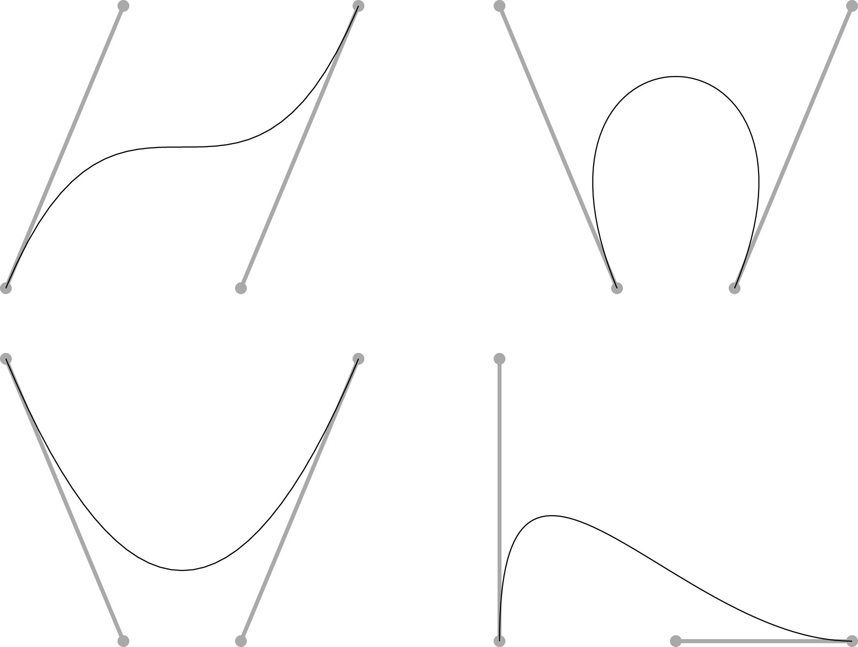
Cubic Bézier Curves
Coordinate Transformations
In Transformations, we saw that we can use tranformation operators to change the current user space. In this chapter, we will pursue this observation is a bit more detail.
For convenience, we will refer to coodinates in the default user space as page coordinates. We are going to explore the relationship between coordinates in the current user space and the page coordinates. This relationship is an affine coordinate transformation. Let \((x_u,y_u)\) be a point in the current user space, and let \((x_p,y_p)\) be the corresponding page coodinates. Then
PostScript collects these six paramters into an array, \([a \; b \; c \; d \; t_x \; t_y]\). In PostScript terms, this is called a transformation matrix. It is a compact representation of the following augmented matrix:
Since the last column of the agumented matrix is constant, its elements are discarded in the compact array reprsentation. If we work with augmented arrays (appending \(1\) to an ordinary array), we can use matrix mulitplication to represent this transformation.
We will write this as \(q^p = q^u A\), relating the augmented vectors via the augmented matrix. This is a typical reprsentation in the graphics world. The rest of us are more likely to recognize the following decomposition, which we will write \(p^p = M p^u + t\).
An affine transformation has a linear component and a translation component. If we zero out the translation component, we have a linear transformation. Two cases of special interest are scale transformations and rotation transformations. A scale transformation can be represented as
Here \(s_x\) is the rescaling of the \(x\) axis, and \(s_y\) is the rescaling of the \(y\) axis. A rotation transformation can be represented by
This gives a counterclockwise rotation around the origin through an angle of \(\theta\).
We we want to consider the effects of a transformation matrix,
we can use transform and itransform to look at the
transformation and inverse transformation of point.
For example, consider:
0 0 [1 0 0 1 72 72] transform
The pushes 72 72 on the ostack, telling us that that the origin in user space is at \((72,72)\) in page coordinates under this transformation. Evidentally, this is reporting (without the never-changing constant) the result of the multiplication
We can find the inverse of this transformation with the invertmatrix_ operator, which takes as operands a PostScript matrix to invert and a PostScript matrix to fill with the result. The matrix operator produces an identity matrix, and we will use this to get a matrix to fill. After executing
[1 0 0 1 72 72] matrix invertmatrix
we find [1 0 0 1 -72 -72] at the top of the stack. Usually we have no need to produce an explicit inverse matrix, since the itransform_ operator works like the transform_ operator but produces an inverse transformation.
Concatenation
Suppose we implement one affine tranformation and then another one. The result is another affine transformation. We can represent this result as the concatnation of the two affine transformations.
A sequence of transformations is easy to implement, but unless they are all linear, the representation qickly gets a little messy. Now consider the the same sequence of transformations represented in terms of augmented vectors and augmented matrices.
This matrix-multiplication representation of the concatenation of affine tranformations is clean and convenient.
We can do multiplication of PostScript matrices with the concatmatrix_ operators, which takes three operands: two PostScript matrices to multiply, and a third to hold the result. Try entering the following at the Ghostscript command line, and explain the difference in the results.
0 0 [1 0 0 1 288 396] [10 0 0 10 0 0] matrix concatmatrix transform ==
0 0 [10 0 0 10 0 0] [1 0 0 1 288 396] matrix concatmatrix transform ==

0 0 matrix defaultmatrix transform pstack
Let's create a procedure to show us where on the page a point in user space lies. A first thought about how to do this would probably be the following: push the coordinates on the stack, push the currentmatrix on the stack, and transform the point. For example,
0 0 matrix currentmatrix transform
This is the right basic idea, but it returns the coordinate in device space. The are the coordinates used by the actually rendering device, which need not match our page coordinates. So we now encounter another coordinate space: device space. The tranform of page coordinates to device coordinates provided by the defaultmatrix_ procedure. To go from device coordinates to page coordinates we need the inverese of that transform. So we end up with the following:
/pageLocation {matrix currentmatrix transform matrix defaultmatrix itransform} bind def
Similarly, we can determine what user coordinates correspond to a particular point on the page.
/userLocation {matrix defaultmatrix itransform matrix currentmatrix transform} bind def
More Programming in PostScript
Scope
Sometimes we want to use a name without overwriting any pre-existing value.
For example, we may want a variable name to be local to a procedure.
We can use a dictionary to limit the variable scope in this fashion.
A dictionary of names and associated values can be put on the operator stack
by bracketing these pairs with << and >>. [28]
This dictionary can then be popped from the operand stack
and pushed onto the dictionary stack with the begin operator.
When we are done with it,
we pop it from the dictionary stack with the end operator.
| [28] | The << operator pushes a mark object on the ostack,
while >> operator creates a dictionary from the key-value pairs following the nearest mark.
Like the [ operator,
the << operator is a synonym for mark.
By convention, we use << for our dictionary definitions. |
As an example, we can rewrite our factorial procedure in a more traditional way, using a variable and a for loop.
/factorial {    % n
  1 1 1         % n 1 1 1
  4 -1 roll     % 1 1 1 n
  {mul}for      % n!
} bind def
Of course this code looks rather ugly and inefficient after seeing the stack oriented approach above,
but it does illustrate how a dictionary can be used by a procedure to limit the scope of a variable.
The code has another pedagogical advantage as well:
it effectively illustrates the difference between an executable name and a literal name.
When the PostScript interpreter encounters the name nfac,
it executes it.
That is, it pushes on the ostack the value associated with it in the current dictionary.
In contrast, when it encounters /nfac,
it pushes on the ostack the literal name,
to which we then assign a new value using the def operator.
This updates the value of nfac,
so each iteration through the for loop that value has changed.
Recursion
PostScript supports recursion (including tail call elimination), but it must be handled carefully. As in other languages, it is often simplest to rely on iterative equivalents of recursive algorithms. When a recursive algorithm with variables is for some reason desirable, you will need to carefully attend to variable scope. As a classic example, the following procedure fails because it does not localize the scope of the variable name.
/RDstackFailFactorial {
  /n exch def      %ooops! all calls will use same def!
    n 2 lt
    {1}
    {n 1 sub RDstackFailFactorial n mul} %bad 2nd val for n
  ifelse
} def
Exercise
For integer valued \(n\),
explain why n factorialDstackFail always produces 1 instead of \(n!\).
Instead, we need each recursive call to create its own dictionary on the dictionary stack and to remove it (with end) when done with it. Recall that names are resolved by looking down the dictonary stack until the name is first found.
/RDstackOKFactorial {
  1 dict         % create new local dict for 1 entry
  begin          % push it onto the dictonary stack
  /n exch def    % establish name n in new dict
    n 2 lt
    {1}
    {n 1 sub RDstackOKFactorial n mul}
  ifelse
  end            % pop the new dict
} def
This still has a couple of problems. First of all, the allowabe depth of the dstack is implementation specific. (Early implementations of PostScript only allowed a depth of 20!) Second of all, lookup on the dstack is relatively slow.
So we usually use the ostack instead of the dstack. The maximum depth of the ostack is also limited, but even early interpreter implementations typically allowed 500 operands. Modern implementations may allow tens of thousands of items on the ostack. Consider the following code, which implements a standard recursive algorithm for computing the factorial of a positive integer. [29]
Branching
The branching operators are if and ifelse. The if operator requires two operands: a boolean and a procedure. If the boolean is true, the procedure is executed. The ifelse operator requires three operands, a boolean and two procedures. If the boolean is true, the first procedure is executed. Otherwise the second procedure is executed.
As an example, consider the following line of code:
true {1}{0}ifelse
The boolan is true, so the first procedure is executed
(and the second is not).
The first procedure is trivial:
it simply pushes 1 on the ostack.
| [29] | A good introduction to algorithms is [cormen.leiserson.rivest-1990-mit]. |
% int *ROstackFactorial* int
%                 %with ostack(... n) where n>1
/ROstackFactorial {
  dup             % n n
    2 lt          % n true
    {pop 1}       % n true proc
    {dup 1 sub ROstackFactorial mul}  % n true proc proc
  ifelse          % n*(n-1)! (*after* (n-1)! returns)
} def
The procedure duplicates the top object on the ostack. (A more careful implementation would check that this object is a positive integer, which is required for this procedure to work correctly.) Let us call the number on the top of the ostack \(n\). The duplicate of \(n\) is used to test whether we have a number less than \(2\). If we do, the boolean true is pushed on the stack. Two procedures are then pushed on the stack If the ifelse operator sees the value true, it executes the first procedure in the inner braces. This just replaces \(n\) with \(1\) on the ostack. Otherwise, it executes the second procedure. This copies the number, subtracts one from it, computes \((n-1)!\), and multiplies \(n\) times \((n-1)!\). Note how reliance on the stack means that we used no variables in this procedure.
As a reminder, this approach still accumulates many items on the ostack. We can easily avoid this with a less elegant but cheaper implementation.
/factorial {    % n
  1 1 1         % n 1 1 1
  4 -1 roll     % 1 1 1 n
  {mul}for      % n!
} bind def
Sorting
Ghostscript ships with a bubble-sort implementation named .sort.
See: https://en.wikibooks.org/wiki/PostScript_FAQ#How_to_sort_an_array.3F for a PostScript sorting implementations.
See [casselman-2005-cup] ch. 9, which offers a quicksort implementation and applies it to the convex hulls problem.
Custom Stack
It is possible to use an array as a stack.
See line 45 of dr00g's https://github.com/luser-dr00g/ibis.ps/blob/0c0aa7d5bd683d21d9814b2b697a85028bcddc81/ibis.ps#L45
Debugging
Support for debugging is a PostScript weakness.
See: https://en.wikibooks.org/wiki/PostScript_FAQ#How_to_debug_a_PostScript_program.3F
Adding Your Drawing to a Document
Format Conversion
Format conversion using Ghostscript.
- From: http://wwwimages.adobe.com/content/dam/Adobe/en/devnet/pdf/pdfs/PDF32000_2008.pdf
- This postfix notation, in which an operator is preceded by its operands, is superficially the same as in the PostScript language. However, PDF has no concept of an ostack as PostScript has.
Nevertheless, PDF does provide for what are PostScript calculator functions. These are pure numerical functions with no side effects, computed using familiar PostScript operators.
Adding Text to a Drawing
Until now, we have entirely neglected the topic that is the main focus of most introductions to PostScript: the placement and manipulation of text. Since this booklet focuses on PostScript drawing, so we will have little to say about adding text. Indeed, if you need to add more than a minimal amount of text to your drawings, it is probably most efficient to use an application that allows you to import your PostScript drawing and annotate it.
For simple labels, however, you may wish to include the text for your drawings in your PostScript Program. Conceptually this is simple.
- Select your font.
- Place your text at a specified location.
- “Print” the text on your drawing.
Choose Your Font
In principle you can use any PostScript, TrueType, or OpenType font to add text to your PostScript drawings. [30]
| [30] | As long as you have access to a LanguageLevel 3 interpreter. |
For occasional drawing, however, the practical options are a fairly small set: you will want to use fonts that you can be confident are present in every PostScript interpreter that might be used to render your drawing. The original Apple LaserWriter (1985) had 13 built-in fonts: the Times, Helvetica, and Courier font families, plus the Symbol font. [adobe-1999-plrm3] [p.773] considers these to be “standard”. You can expect that any PostScript interpreter will have access to fonts using these names. Indeed, a superset of 35 fonts can be considered standard: add the Bookman, Palatino, New Century Schoolbook, Avant Garde, and Helvetica Narrow families, (this last being a simple rescaling of Helvetica to .82 of its usual width) along with Zapf Chancery Medium Italic and Zapf Dingbats. Adobe considers 136 fonts to be “core” in Adobe PostScript 3, but unless you know ahead of time which fonts will be available where your PostScript drawing will be interpreted, it is best to stick to the basic set of 35. [31]
| [31] | However Helvetica is risky if you care about the precise appearance of fonts in your drawings: to avoid licensing fees, Arial is often substituted when Helvetica is requested. (Even Adobe Acrobat does this now. The easiest visual test is to look for Helvetica's “spur” on the capital G.) You can of course ask your interpreter to use any new fonts that you acquire. For example, in Ghostscript you just add the font name and the location of the file with the font information to Ghostscript's Fontmap file. |
The Adobe PostScript fonts typically come in families of four. The four members of the Times family are Times-Roman, Times-Italic, Times-Bold, and Times-BoldItalic. The Helvetica family comprises Helvetica, Helvetica-Oblique, Helvetica-Bold, and Helvetica-BoldOblique. The four members of the Courier family are Courier, Courier-Oblique, Courier-Bold, and Courier-BoldOblique. Some specialty fonts such as Symbol are not part of a family. At four typefaces for each of the eight families plus the three additional fonts we get a standard set of thirty-five fonts. [32]
| [32] | Here are the rest: AvantGarde-Book, AvantGarde-BookOblique, AvantGarde-Demi, AvantGarde-DemiOblique, Bookman-Demi, Bookman-DemiItalic, Bookman-Light, Bookman-LightItalic, Helvetica-Narrow, Helvetica-Narrow-Oblique, Helvetica-Narrow-Bold, Helvetica-Narrow-BoldOblique, Palatino-Roman, Palatino-Italic, Palatino-Bold, Palatino-BoldItalic, NewCenturySchlbk-Roman, NewCenturySchlbk-Italic, NewCenturySchlbk-Bold, NewCenturySchlbk-BoldItalic, ZapfChancery-MediumItalic, ZapfDingbats. In fact there are usally more fonts available: https://partners.adobe.com/public/developer/en/ps/PS3010and3011.Supplement.pdf lists 136 different fonts as “typically” available. |
Once you decide on a font face and size, you are ready to go. Just use the selectfont operator to select the font and font-size. For example, /Helvetica 25 selectfont sets the current font to Helvetica at 25 points.
Placing Text
To place text in your drawing,
you need to create a string that contains the characters to be painted.
The easiest way to create a string is by enclosing a set of characters in matched parentheses:
(this is a string). [33]
| [33] | A string can also contain matched parentheses,
but unbalance parentheses must be escaped: \( or \).
Backslashes must also be escaped in strings: \\.
Other escape sequences for strings are less used: \r, \n, \f, \t, \b, \nnn. |
The current point determines the placement of the lower left corner of your text when the string is “printed." Set the current point to where you wish your text to begin.
Note that when we quote a literal string object with parentheses,
as with (Hello World),
this does not print anything.
Until we know what font we will use,
it does not even tell us what will appear when we print.
It is just a way to produce a sequence of character codes,
which different fonts (e.g., the Symbol font) may interpret differently.
"Printing” Text
To print your string, use the show operator. The show operator takes one operand, a string. The show operator also requires that the current point and current font be defined. It prints the string in the current font, with the lower left corner at the current point. After the text has been printed, the current point is at the lower right of the string. As an example, to print the text “Print this." in 40 point Helvetica starting at the center of a sheet of letter paper we could use the code
%!
/Helvetica 40 selectfont     %select your font
306 396 moveto               %move to center of page
(Print this.) show           %print “Print this.” on the page
showpage                     %view your work
Aligning Text
The example above drives home the point that only left alignment of text is automatic in PostScript: the show operator begins painting text at the current point. To center text at a position, we need to shift the current point to the left of that position by half the width that text will occupy. We can obtain that width with the stringwidth operator, and we can produce the necessary relative movement with the rmoveto operator. As we saw in the section on Relative vs Absolute Positions, the rmoveto operator takes as operands the horizontal and vertical displacements (dx,dy) relative to the current point.
For centered text in the above example, you can precede the show operator with
dup stringwidth pop -2 div 0 rmoveto
This gets the string width, divides it in half, and moves the current point left by the resulting amount. (patterns01 uses this code to center single characters (the numbers) inside a polygon.) Right justification to the current point is achieved similarly:
dup stringwidth pop neg 0 rmoveto
In both cases, the use of the stringwidth is supplemented by two additional operators that you may not have expected: the stack manipulation operators dup and pop. These are needed because stringwidth consumes its operand and leaves an extra item on the operator stack. The dup operator duplicates the string for use by the the stringwidth operator, and the pop operator pops the superfluous item from the ostack.
The Symbol Font
The standard PostScript font set does not support serious mathematics. Of course one can purchase specialized font sets, but even then it is best to rely on an application (such as LaTeX) for the typesetting of complex mathematics.
Occasionally however it is useful to place a few mathematical symbols or Greek letters on a drawing, and the standard Symbol font can often be used for this. The character names and character codes of this font are documented in Appendix E.12 of [adobe-1999-plrm3]. For occasional use, it is helpful that the characters can be accessed with the glyphshow operator, which allows you to work directly with the character name (in the current font). For example, the following code places the text ∑ α on the page.
%! /Symbol 40 selectfont %select Symbol font at 40 points 306 396 moveto %move to middle of page /summation glyphshow %print a summation sign on the page /alpha glyphshow %print a Greek alpha on the page showpage %view your work
We do not have to use glyphshow:
we can use the character codes in a string with the show operator to achieve the same effect.
For example, α has character code 141 and ∑ has character code 345 in the Symbol font,
so the more compact (\345\141)show would also have painted the same text on the page.
However for occasional drawing using the Symbol font,
it is wiser to use the character names,
as these aid in understanding and debugging your PostScript programs.
Adding Text with PyX
PyX does EPS import (and is workingon PDF import). Note that PyX (v.0.14) does not directly support TrueType fonts, but the FAQ offers a work around for this. The discussion of this section assumes you will use the default (Computer Modern) TeX fonts.
Create your EPS figures. Import them into PyX, and add whatever text you wish.
Ask PyX to export as EPS, and use Ghostscript to convert the format to PDF. You should reliably end up with a vector graphic this way.
Clipping and Pattern Fills
In sections First Steps, Transformations, and `Circles and Rectangles`_, we created simple drawings in two steps:
- Construct a path.
- Paint the path (i.e., stroke or fill it).
That is the simple essence of PostScript drawing. This section provides some additional details about these two steps, with an emphasis on the utility of dashed lines.
Dashed Lines
Economists use dashed lines in their drawing almost as often as solid lines. Fortunately, PostScript makes painting a dashed line as simple as painting a solid line along any path. The key to this is the setdash operator.
The setdash operator takes two operands:
an array of numbers that determines the dash pattern,
and a number that determines the setdash offset for this pattern.
The array is just a list of numbers surround by brackets.
The numbers determine the dash lengths and gap lengths along a stroked path.
For example the array [5] indicates a dash of 5 units followed by a gap of 5 units.
(Note that the stroke operator “cycles” through the array.)
As another example the array [5 1] indicates a dash of 5 units followed by a gap of 1 unit.
There is no restriction the length of this array, so very complex dash patterns can be specified.
The dash pattern is repeated along the entire stroked path.
The offset operand determines how far “into” the dash pattern we are at the beginning of the stroked path.
For example, after [5] 5 setdash,
a stroke operation would begin with a gap of 5 units.
whereas after [5] 2 setdash,
a stroke operation would begin with a dash of 3 units.
In section Transformations we learned how to construct equilateral triangle and, by implication, regular polygons with any number of sides. In patterns01 we use that knowledge to construct six pentagons, which we stroke or fill in various ways. In every case we make use of dash patterns.
The simplest case is pentagon 1. Any path we can construct we can also stroke with a dashed line. We illustrate this by stroking pentagon 1 with a line width of 2 after the instruction [15] 0 setdash. This dash pattern starts with a dash of 15 units, followed by a gap of 15 units. That initial pattern is then repeated around the entire pentagon.
Clipping Path
What happens if you stroke or fill a path that you have constructed in such a way that it goes beyond the boundaries of the page? The answer probably seems very natural: only the part of your drawing that is within the page boundary is painted. Anything beyond that boundary is “clipped": it has no effect on the drawing.
Part of the graphics state is the clipping path. (See gstate and clip.) While this is initially the page boundary, it can be constrained further by any path you might wish to construct. Simply construct the path and then invoke the clip operator. From then on, any painting will take place only within the new clipping path. You can do this as many times as you want, but the operation is one of repeated intersection: the clip operator can only reduce the area enclosed by the clipping path. If you need to temporarily shrink the clipping path, then you need to save and restore the larger path. Traditionally this is done by saving and restoring the entire graphics state with gsave and grestore, as discussed in Color. [34]
| [34] | However modern PostScript implementations include the clipsave and cliprestore operators that may be used instead. Use these operators only if you are sure your PostScript files always have access to interpreters that adequately support LanguageLevel 3. |
Bracketing every change to the clipping path between a gsave and a grestore is a reasonable practice, which we follow in this section.
Consider pentagon 2 in patterns01. This illustrates our first use of the clip operator. We are going to add “tic marks” to the inside of the pentagon, since this is one common method of highlighting a specific region. After constructing a pentagon shaped path, we proceed as follows.
gsave                 %save the graphics state
clip                  %clip to current path
[2 25] 12 setdash     %set dash pattern and offset
10 setlinewidth       %thick width produces “tics"
stroke                %stroke the “tics"
grestore              %restore the graphics state
stroke                %stroke path with solid line
First we save the graphics state, which includes our current path and clipping path. (Recall that the current path is the pentagon that we constructed.) We clip to this path so that any painting will take place only inside it. We then set a dash pattern: here we somewhat arbitrarily pick a 2 unit dash followed by a 25 unit gap. When we set the thick line width of 10 units and stroke the pentagon, our dashes show up as “tics” on the interior of the pentagon. Note how the dash length effectively appears as the line width of the tics. Note also how the clipping path restricts the painting to the interior: without this clip operator these tic marks would extend equally on both sides of our path. (Try it!) Of course the stroke operator issues an implicit newpath operation, thereby destroying our constructed pentagon. However since this path was part of the graphics state when we used the gsave operator, we can restore it with the grestore operator. After restoring our constructed pentagon as the current path, we stroke it. Since the dash pattern and line width are part of the graphics state, this stroke operation uses their original values. The grestore operation similarly restores the original clipping path, so we get the full line width when we stroke our pentagon. The result is pentagon 2 in patterns01.
Pattern Fills
Economists' drawings often contain shaded areas, where the shading follows a variety of conventions. Section Color_ discussed how arbitrary paths can be filled with arbitrary colors, including arbitrary shades of gray, and this is one common approach to shading. This section discusses some alternatives to such color fills.
Color fills are currently the best choice of shading for electronic documents, since the resolution of computer monitors is inadequate to effectively display most pattern fills at standard magnifications. For the moment, economists should generally reserve their use of pattern fills for print media.
PostScript is capable of tiling the inside of an arbitrary path with an arbitrary pattern. This facility goes far beyond the needs of occasional drawing is beyond the scope of this booklet. [35]
| [35] | For good discussions see section 4.9 of [adobe-1999-plrm3] or especially ch.11 of [mcgilton.campione-1992-psxmpl]. |
However certain simple pattern fills are common in economic illustrations. For example, hatching and cross-hatching are often used by economists to shade regions of a drawing. [36]
| [36] | For randomly chosen illustrative examples from textbooks and journal articles see ch.3 of [beavis.dobbs-1990-cup], [glaeser.shleifer-2002-qje], [lucas.rossi-2002-e], or section 1.18 of [varian-1984-norton]. |
This section shows how to produce simple pattern fills simply by using very wide dashed lines.
Hatching
For example, consider the hatching that fills pentagon 3 in patterns01. What we learned in section First Steps about drawing line segments and in section clippath_ about clipping suggests one straightforward approach to producing such hatching: clip to the pentagon, repeatedly construct thin line segments passing through it, and then stroke the resulting path. While this works fine, a much simpler solution exists. We will still clip to the pentagon, but we then paint a single very wide dashed line passing through it. If the current origin is at the center of a constructed pentagon that has a 1.5 inch “radius", then after clipping to the pentagon we can construct this path as follows.
newpath                  %start a new path
-108 -108 moveto         %start path at lower left
108 108 lineto           %construct line to upper right
216 setlinewidth         %very wide line width
[2 20] 0 setdash         %set narrow dash with wide gap
0.5 setgray              %set color to medium gray
stroke                   %stroke the line segment
Note the use of the newpath operator: in contrast to the previous example, we do not wish to stroke the path of the pentagon, which is not destroyed when we clip to it. The next few steps work with some very rough approximations in determining path location and line width. These approximation are harmless because nothing outside the clipping path will be painted. The underlying idea is this: if we surely fill an encompassing region, then we will surely fill the pentagon. There is no need for this encompassing region to be small since only the inside of our pentagon will be painted: nothing prevents us from letting the encompassing region be the entire page!
In this case we construct an upward sloping line segment right through the center of our pentagon. The line -108 -108 moveto moves to the lower left corner of an encompassing square. The line 108 108 lineto constructs a line segment to the upper right corner of this encompassing square. The line 216 setlinewidth makes sure that the line is wide enough when stroked to completely encompass our encompassing square. If we were to stroke our constructed line segment at this point, it would completely fill our pentagon with black.
Instead we give the instructions [2 20] 0 setdash which sets a dash pattern of 2 unit of dash followed by 20 units of gap. We can now stroke our line segment and it will fill our pentagon with hatching that is perpendicular to our constructed path. Before we do so, however, we change the current color to a medium gray, since gray hatching has more visual appeal than black. The important thing to note is that the apparent line width of the hatching is actually the dash length of 2 units.
It is hard to imagine a simpler way to generate exactly practically any desired hatching pattern. [37]
| [37] | As a point of comparison, consider how easy this technique makes it to produce the 16 predefined hatching patterns in the NCAR graphics command language. (As well as many others, of course.) |
The “line width” of the hatching and its angle can be easily varied in the obvious way: change the dash pattern and the angle of the constructed line segment. Similarly, if cross hatching is required, just construct a second line segment through the pentagon before the stroke operation. In order to stress the ease of such changes, we produce the patterned hatching that fills pentagon 4 by changing a single line of code: the dashing pattern is set by the instructions [2 20 2 5] 0 setdash.
Stippling
Stippling is another widely used pattern fill. Using dash patterns we can produce a variety of stippling effects very simply. The core idea is to fill an area with the stippling color, then cross hatch the area with thick white lines. Black stippling is illustrated in pentagon 5 in patterns01. [40]
| [38] | Like other graphics decisions in this booklet, the very large stipples are chosen to permit display on relatively low resolution computer monitors. If you are viewing this with a monitor that nevertheless cannot display the stippling, try zooming in on the figure.} |
Once again, let the current origin be at the center of a pentagon that has a 1.5 inch “radius", After constructing the pentagon and clipping to it, the stippling can be produced with the following code.
0 setgray fill           %black filled pentagon
-108 -108 moveto         %start path lower left
108 108 lineto           %construct line to upper right
108 -108 moveto          %start subpath lower right
-108 108 lineto          %construct line to upper left
216 setlinewidth         %set very wide line width
[20 10] 0 setdash        %set dash pattern and offset
1 setgray                %set color to white
stroke                   %stroke the line segments
Since this is very similar to the previous example, let us focus on the differences. The first line has been changed to 0 setgray fill. This fills the pentagon with black. Recall from section Colors that a fill operation performs an implicit newpath operation, so we can drop that instruction from our code. We next begin path construction just as in the previous example, drawing a line segment with unit slope through the center of the clipped pentagon. Let us call this segment 1. Then we add a new segment to our construction: this is perpendicular to segment 1 and also extends through the clipped pentagon. Let us call this segment 2. As before, we pick a line width that “encompasses” the clipped pentagon. If we were to stroke our path at this point, it would cause no visible changes: we already have a filled black pentagon. However if we first change the current color to white with the instructions 1 setgray, then stroking our path would produce (because of the large line width) a filled white pentagon. The trick is to change the current color to white and change the dash pattern. We use a dash pattern of [20 10] 0 setdash, which paints a 20 unit dash followed by a 10 unit gap. When we paint this in white along segment 1, it paints thick white hatching over our black pentagon. When we continue painting along the perpendicular segment 2, we have effectively painted thick white cross hatching over our black pentagon. The visual appearance, however, is the stippling in pentagon 5 in patterns01.
This basic structure again allows the ready production of many different pattern fills. For example, try making just two small changes: fill the pentagon with red instead of black and change the dash pattern to [1 10] 0 setdash to get a widely used (and radically different) pattern fill. (Be sure to predict the outcome before looking at it.)
Just for Fun
Color fills, hatching, and stippling should be adequate to the shading needs of most economists. Nevertheless we will briefly explore a simple way to produce the “checkerboard” shading in pentagon 6 in patterns01. As a shading exercise, this is pure entertainment. However it serves the more serious purpose of introducing two final PostScript operators: strokepath and especially eofill.
The strokepath operator replaces the current path with, roughly, the “outline” of the shape that would result from stroking it given the current graphics state. For example, in the default graphics state, applying strokepath to a line segment will produce a rectangular path whose width is the line width. When we apply the strokepath operator to a dashed line, we get a path consisting of outlines of the dashes.
The eofill operator behaves just like fill operator with one exception: it uses the even-odd rule to determine which points are inside the current path. To apply the even-odd rule to a point, draw a ray from that point in any direction and count the number of times you cross the current path. If that number is odd, the rule says that point is inside the path. For example, if we construct a path that is two circles, points in the interior of both circles are not “inside” the path, whereas points interior to only one circle are considered “inside” the path. [41]
| [39] | This makes Venn Diagram illustration of the concept of “symmetric difference” trivial.} |
We now use the strokepath and eofill operators together to produce the "checkerboard” shading in pentagon 6 in patterns01. The strategy is very similar to our previous pattern fill, and indeed much of the code is the same. Once again, let the current origin be at the center of a pentagon that has a 1.5 inch “radius", recalling 1.5 inches is 108 points. After constructing the pentagon and clipping to it, the checkerboard can be produced with the following code.
newpath
-108 -108 moveto         %start path lower left
108 108 lineto           %construct line to upper right
108 -108 moveto          %start subpath lower right
-108 108 lineto          %construct line to upper left
216 setlinewidth         %set line width very wide
[36] 0 setdash           %set dash pattern to 0.5" bands
strokepath               %set path to outline of bands
0.5 setgray              %set current color to gray
eofill                   %paint points inside a single band
As in our hatching examples, we need to begin with a new path. The subsequent path construction is identical to the stippling example: we construct perpendicular diagonals through the center of the pentagon. Once again we pick a path width easily wide enough to “encompass” our pentagon. Along the constructed path, the instructions [36] 0 setdash will therefore create a very thick cross-hatching within the pentagon. A single “dash” will be painted as a half inch wide diagonal whose slope will be plus or minus unity (along the second or first line segment). The strokepath operator will create the outline of these bands. The important point is that every point in the pentagon will fall within either 0, 1, or 2 of these bands. The eofill operator will only paint those points that fall inside a single band. This creates the checkerboard appearance.
Needless to say, many variants are possible. Changes in the dash pattern or the angle at which the line segments pass through the pentagon can produce many pleasing pattern fills. While this serves to illustrate the power and simplicity of PostScript, the eofill operator was the most important concept introduced in the present section.
Other Stacks
We have already talked about the operand stack (or ostack). The ostack stack holds every operand we push on the stack, and so it holds the results of intermediate operations until they are consumed. There are three other stacks used by the PostScript interpreter: the dictionary stack (or dstack), the graphics-state stack, and the execution stack. Each stack embodies limitations (e.g., on the number of elements that may be stored), but our programs will not test these.
When we create a dictionary, it goes on the dictionary stack. Recall that a dictionary is a list of key-value pairs. If we use a name that the PostScript interpreter does not recognize, it tries to look it up a a key in the dictionary stack, starting with the top dictionary. If it finds a key, it will fetch its value. We can use this value like any other.
Keys usually a name type,
but they may be of any type (except null).
Names are unique, case-sensitive identifiers.
These identifiers may name variables or procedures.
They are not strings.
Two dictionaries are always present:
systemdict and userdict.
- systemdict
- holds define the built-in PostScript operators; always at the bottom
- userdict
- holds variables and procedures of a PostScript program; always above the systemdict
The systemdict and userdict cannot be removed from the stack. There may also be a dictionary of fonts or other interpreter specific dictionaries. Most important to us, we can use begin to push additional dictionaries on the dictionary stack and end to pop them off. We create a dictionary on the ostack, and then use begin to pop it from the ostack and push it on the dictionary stack. The topmost dictionary in the dictionary stack sets the current context for any key lookup.
When the interpreter looks up a name, it searches the dictionaries from the top down. The userdict is always searched before systemdict, so you can redefine the built-in PostScript operators. (We won't be doing this.)
The graphics-state stack stores graphics states. At the top is the current graphics state, which stores the current state of graphical elements, such as the current line width, current font, current color, and current path. At any time, we can use gsave to push a copy of the current graphics state onto the graphics state stack, and then we can use grestore to restore it (popping off the current graphics state).
The ostack, dictionary stack, and graphics state stack are under user control: a PostScript program can manipulate them at will. The execution stack is different: we can push objects onto it (e.g., with exec, run, stopped_, for, ifelse, and forall), but otherwised it is manipulated only by the interpreter. The execution stack holds executable objects, such as procedures and files that are currently being executed. Whenever the interpreter interrupts the execution of a current object, it puts the interrupted object onto this stack. It stays there until it is completely executed; then it is removed from the stack. Execution continues with the executable object that is now top-most on the execution stack. We will not disucss the execution stack any further.
Encapsulated PostScript
The focus to this point has been the production of single page PostScript drawings. Come publication time, the publisher will usually request that your PostScript drawings be submitted as Encapsulated PostScript (EPS) files or converted to PDF. A similar need arises if the drawing is for inclusion in a presentation or in another document. [42]
| [40] | Tools to convert from EPS to other graphics formats are widely available. The mostly widely used free conversion tool is probably pstoedit. |
For example, the drawings in this booklet are created as EPS files. Fortunately, it is very simple to turn single-page drawings into Encapsulated PostScript.
Conversion by hand is easy, as we discuss below,
but there is an even easier way:
the free ps2eps converter.
For example, if you have installed GSView (or its equivalent),
just open your single-page PostScript drawing and pick File/PS_to_EPS from the menus.
This produces an EPS file suitable for inclusion in larger documents. [43]
| [41] | It is important to understand that many WYSIWYG applications, such as those in popular office suites, have imperfect onscreen display abilities for inserted EPS files. (For example, Microsoft Word could not do this until Word 2002, and even then its rendering was flawed.) If you need onscreen display in such an application, you will need to add a “preview” to your EPS file. Add a preview with pstoedit. (For ease of use, GSView allows this by means of its Edit menu.) Use of the TIFF 6 file format for the preview provides color and good portability, although applications that do not support this preview may object to it, since it is included as part of the EPS file. The so-called Interchange (or EPSI format) provides a grayscale preview as a series of EPS comments, so it is fully portable. Unfortunately, in practice some applications may ignore the Interchange preview. Rely on applications that have good PostScript support.} |
If you open this EPS file in a text editor, it will look much the same as your original PostScript file, aside from a few new comments. Usually only two of the new comments are absolutely necessary. The first of these says that the document is an EPS file: %!PS-Adobe-3.0 EPSF-3.0. More specifically, the comment has two parts. The first part says that the document conforms to Adobe's Document Structuring Convention version 3.0, and the second says that that it conforms to Adobe's EPS specification version 3.0. This special comment should be the first line in your EPS file.
The second required comment provides a bounding box for your drawing. A bounding box specifies the lower-left and upper-right corners of the smallest rectangle that fully encompasses your drawing, so the form of the comment is: %%BoundingBox: llx lly urx ury. (Coordinates are of course in points and must be integer valued.)[#]_
| [42] | The restriction to integer values can be found on p.39 of [adobe-1999-dsc],
the main document structuring manual.
Non-integer values can additionally be specified with the
%%HiResBoundingBox comment, as discussed on p.6 of [adobe-1999-dsc]. |
For very simple drawings, computing the bounding box by hand is feasible. (One could even print the drawing and use a ruler.) Usually, however, it makes sense to depend on a PostScript to EPS converter to calculate the bounding box.
Note that the first special comment does not refer to the LanguageLevel, and it should only appear in DSC compliant documents. If you want to be very careful, there are two more comments that are technically required in many drawings [adobe-1999-dsc]. Encapsulated PostScript is part of Adobe's Document Structuring Convention (DSC), which is a set of rules for adding special comments to PostScript files. These comments help applications work with the PostScript files. The DSC mandates specifying the LanguageLevel of the drawing and indicating which resources (e.g., fonts) that the drawing requires. In practice, many EPS files lack this information, and most applications will not demand this information. Nevertheless, a brief discussion follows.
Occasionally, PostScript drawings may need one of the newer PostScript operators,
in which case the DSC requires a comment stating the LanguageLevel.
For example, selectfont is a LanguageLevel 2 operator and is very commonly used.
The rectstroke, rectfill, and glyphshow operators are also LanguageLevel 2.
Use any of these should be signalled by the comment %%LanguageLevel: 2.
Similarly, clipsave and cliprestore are LanguageLevel 3 operators,
so use of these you must be signalled by a %%LanguageLevel: 3 comment.
While there are many other LanguageLevel 2 and LanguageLevel 3 operators,
all listed in [adobe-1999-plrm3],
the six just mentioned are the most likely to be used for occasional drawing.
PS to EPS converters do not reliably add a LanguageLevel comment;
plan to provide this comment yourself.
For example,
suppose you have created a drawing that uses the selectfont operator
(which is a LanguageLevel 2 operator)
to select the Times-Roman and Helvetica-Oblique fonts.
Suppose also that your drawing is fully encompassed by a rectangle that extends
from the point (1 inch,2 inch) to the point (3 inch,4 inch),
Then to make an EPS file,
add the following comments to the top of the PostScript file.
(A DSC comment can continue onto multiple lines by using the %%+ comment.)
%!PS-Adobe-3.0 EPSF-3.0
%%BoundingBox: 72 144 216 288
%%DocumentNeededResources: font Times-Roman
%%+ font Helvetica
%%LanguageLevel: 2
In sum, converting PostScript to Encapsulated PostScript is generally rather easy. The absolutely necessary changes are two: change the special comment on the first program line, and add a bounding box. Additionally, to conform to the DSC, specify the LanguageLevel and indicate any resource needs (e.g., fonts used). Generally the applications that import your drawing will take steps against any common mistakes or omissions, but there are still a few crucial rules that an EPS file must follow: [44]
| [43] | As you gain experience with PostScript,
you should attend to a couple more details.
These boil down to efforts to leave the stack and the graphics state in the position it was in before the EPS file was interpreted.
It is a good idea to make sure your EPS files does not leave anything on the stack.
It is very important that an EPS file not use global graphics state commands.
This proscribes the use of certain PostScript operators,
which are listed in Appendix G of [adobe-1999-plrm3].
(This booklet uses none of the proscribed operators.)
Finally, the obsessive should view the DSC and EPSF specifications
to discover some additional DSC comments that are encouraged,
including the When drawings may be handled by less robust applications, taking a couple precautionary steps may pay off. For example, consider using a private dictionary for each EPS drawing. To be extra careful, consider initializing the graphics state (e.g., by setting the current line width and color) rather than assuming the importing application will initialize to the PostScript default values. However, most applications that import EPS files will be careful enough that these extra precautions will not be necessary. |
- be a single page drawing
- use the special header
%!PS-Adobe-3.0 EPSF-3.0 - specify a bounding box
- do not leave anything on the stack
- do not affect the global graphics state.
Finally, it is worth addressing a point of possible confusion. Some authors recommend that an EPS file should not use the showpage operator, since it instructs the printer to eject the current page. However, standard PostScript to Encapsulated PostScript conversion routines leave this operator in your EPS file. This should be fine: Adobe is quite explicit that any application importing an EPS file should redefine showpage so that the EPS file does not actually eject the page.
Including EPS Files
The basic process to include an EPS file in another PostScript file is the following:
save mark
% include your EPS file here
cleartomark restore
You can literally copy the EPS file content into your PostScript file.
Or if your workflow permits file dependencies,
you can use the PostScript run operator to include the file.
(Use forward slashes for path separators, even on Windows.)
save mark
(myfigures/myEPSfile.eps) run
cleartomark restore
Recall however that many EPS files include a showpage operator,
which instruct the printer to eject a page.
It is wise to disable this by redefining showpage.
save mark
/showpage {} def
% include your EPS file here
cleartomark restore
There are still some details to attend to.
For one thing, you will likely require some
transformation to make it appear in the location, size, and orientation that you want.
As a detail, it is wise to disable the setpagedevice operator.
You may therefore wish to proceed as follows.
(See [deubert-200411-aj36b]) for more details.)
%%BeginDocument
/myOldDocumentState save def
mark
/showpage {} def
/setpagedevice /pop load def
%translate, scale, and rotate as needed
% include your EPS file here
cleartomark
myOldDocumentState restore
%%EndDocument
Finally, on Windows some EPS files include a (TIFF or WMF) “preview” as part of the file, and if it does the file should begin with a 30-byte header of directory information. On the Mac, some EPS files include a preview in the file’s “resource fork”. On other systems, there may be an Encapsulated PostScript Screen Image (EPSI) preview included in the file as a special series of comment lines. This booklet does not explore preview generation. To work in a Windows environment with an EPS file that includes a preview, it is generally simplest to strip off the header and preview.
Images
Grayscale Images
An image is a rectangular array of sample values. The image data is stored as a hexadecimal string: a sequence of character pairs, where each pair represents a number from 0 to 256.
Grayscale images can be produced with the image operator. An image is represented as a sequence of components, where each component represents a sample from the image. You need to specify:
- image width
- image height
- color depth as bits per sample, one of 1, 2, 4, 8, or 12. (Based on number of color components per sample, and number of bits per color component)
- transformation matrix, expressing the transformation from your user space to the source image space
- data source
The image is placed based on its lower left hand corner.
The data source can just be a hexadecimal string, or it can be a procedure. If is it a procedure, it must return a string. If the string is too short, it will be used repeatedly to get all the data needed. If it is too long, the extra data will be discarded. The strings represent the image samples, from left to right, starting at the bottom.
Let us start by considering a simple example:
a black and white image.
We allocate one bit to each sample,
which specifies either black (0) or white (1).
A single hexadecimal character represents 8 bits.
For example, 00 has the bit representation 00000000,
while ff has the bit representation 11111111.
Suppose we want to represent the following image.
10000000
01000000
00100000
00010000
00001000
00000100
00000010
00000001
We need to start at the bottom left and work left to right, then bottom to top.
Note that an entire row can be represented by a single hexidecimal pair.
The first row can be represented by 01, the second row by 02, and so forth until the
representation of the last row by 80.
Our hexidecimal string to represent this figure can therefore be <0102040810204080>,
if we use 1 bit per sample.
So the simplest representation of this figure will be
8 8 1 [1 0 0 1 0 0] <0102040810204080> image
However by default a sample will be represented as a 1 point by 1 point square. So by default, our figure will just be a tiny square in the bottom left of our page. Suppose instead we want to map our image to a unit square located at the bottom left but just inside one-inch margins. One way to do that is to change the transformation matrix from the identify matrix to [1 9 div 0 0 1 9 div -8 -8]. (Remember, it is the tranformation from user space to image space!) Here is a more intuitive way to do the same thing.
gsave
72 72 translate
9 9 scale
8 8 1 [1 0 0 1 0 0] <0102040810204080> image
grestore
This simple figure provides a nice opportunity to explore the role of the color depth argument of image.
If we change this from 1 to 2,
then we will be allocating two bits to each sample.
This allows us to represent four colors:
black (bin00), dark gray (bin01), light gray (bin10), and white (bin11).
Of course if we change the color depth in this way but keep our hexidecimal string unchanged,
it will contain only half the information we need.
But that is alright: it will just be used twice.
With a color depth of two,
one pair of hexidecimal digits no longer represents an entire 8 sample row of a figure.
Instead it only represents half a row.
So if our image changes to 8 8 2 [1 0 0 1 0 0] <0102040810204080> image,
the bottom row is now represent by two hexidecimal numbers (01 and 02).
Let B be black, D dark gray, L light gray, and W white.
Then since hex01 is bin00000001 and hex02 is bin 00000010,
our first row is BBBDBBBL.
If we allocate 8 bits to each sample,
we can support 256 different shades of gray
(from black (0) to white (255)).
To represent all these possible shades,
we can put the associated character codes into a string of length 256,
/mystr 256 string def
0 1 255 {mystr exch dup put} for
Then we can use the image operator to create a 16 by 16
grid of these different shades.
16 16 8 [1 9 div 0 0 1 9 div -8 -8] mystr image
We can also use substrings to create an effective “fountain fill”. Here is an example using 150 different shades.
/fillvals mystr 10 150 getinterval def
gsave
72 72 translate
1 150 scale
150 1 8 [1 0 0 1 0 0] fillvals image
grestore
Of course a given device may or may not display so many shades of gray.
Conclusion
Economists often need to produce simple yet precise drawings. Sometimes drawings that are difficult or tedious to produce in a “point-and-click” vector drawing application are very simple to code after a brief exposure to the PostScript page description language. This booklet provides examples of such drawings. The goal of the booklet is to introduce PostScript drawing in a way that emphasizes tools that are useful for producing the precise geometrical relationships occasionally needed in economic research.
Few economists will turn directly to the PostScript page description language for all of their drawing needs: there are many good applications for data driven graphics, functional representations, and even vector drawing. Each of these can be the right tool, depending on the job. PostScript drawing is best seen as a complement to rather than a substitute for such applications. Three core motivations for turning to PostScript for occasional drawings are precision, speed, and fun. A fourth reason is that occasionally it is necessary to tinker with the PostScript produced by another application.
PostScript is an excellent yet easy to learn tool for the production of simple yet precise representations of geometric relationships. For economists, this proves particularly useful in the fields of social choice, public choice, game theory, and mathematical economics. This booklet illustrates both the simplicity and the utility of PostScript drawing for economic research. The results are often as visually exciting as they are useful.
Arrow Code
Application: Drawing Arrows
We now put a few of these programming concepts to work to create a useful procedure. Economists often need to draw an arrow just as we can draw a line in PostScript: from the current point to a specified endpoint. PostScript does not offer a built in operator for this. The most obvious reason is that the problem of drawing such an arrow is not well specified: there are as many different ideas of what constitutes a nice arrowhead as there are people who have thought about it. Additionally, there is the problem of scaling. An arrowhead that looks nice on a 10 point line may look quite wrong on a 1 point line, despite being appropriately scaled. As can be seen in figure [fig:arrows]_, the following procedure definition produces arrowheads that look good over a reasonable range of line widths. It has also been written to allow easy modification to reflect the tastes of the user. Specifically the relative width of the arrowhead can be set to another value---e.g., a larger value to go with small line widths---or computed based on the current line width. This is a pedagogical implementation, so it has limitations (e.g., in the handling of dashed lines), but it is still very useful.
This sections contains the most complex code in this booklet,
and it has been written to illustrate a few programming possibilities.
We will carefully consider a few of the details.
The object is to define a procedure arrowto that we can use just like we are used to using lineto.
So we begin by pushing the literal name arrowto on the stack, followed by a procedure, followed by the def operator.
In broadest outline, we have /arrowto { ... } def,
where the dots indicate the procedure body.
Of course the procedure body is where we will be doing all our work.
We want the procedure body to construct a line segment from the current point to an endpoint specified by the top two operands on the ostack.
Take a look at the procedure body.
The first thing we do there is start a dictionary by pushing a mark object on the ostack with the << operator.
This dictionary is going to hold all the variable definitions used by our procedure.
Put another way,
we are going to make sure that all the variables in this procedure are strictly local to the procedure.
(It is possible to write this procedure to just use the stack and avoid defining any variables,
but the use of variables will be a great aid to understanding the procedure.)
Our procedure anticipates the presence of two numbers on the top of the ostack,
which are the coordinates of the end point for our arrow.
We will assign these to the variables tipy and tipx in our dictionary.
Once we have pushed a mark object on the ostack with the << operator,
we push the literal name tipy on the stack and roll the y coordinate to the top of the stack.
Then we push the literal name tipx on the stack and roll the x coordinate to the top of the stack.
To see how this works, let us suppose that we are drawing an arrow to the point (72,144) and watch how the stack changes.
(This stack illustration leaves out the transient changes involving the operands for the roll operators.)
144       <<   /tipy    144   /tipx        72
 72      144      <<  /tipy     144     /tipx
 --       72     144     <<   /tipy       144
 --       --      72     72      <<     /tipy
 --       --      --     --      72        <<
The crucial thing to notice is that the mark object can be manipulated on the ostack like any other object. Thus we can use the roll operator to move the endpoint coordinates above the mark, so that each can be used as the value of a name-value pair. The dictionary we will therefore associate the value 72 with the name tipx and the value 144 with the name tipy.
We continue to accumulate name-value pairs on the stack in this fashion.
Note that the currentpoint operator pushes on the stack two values representing the current point.
The exch operator is a stack manipulation operator that switches the order of the top two objects on the ostack.
Note that while the mark object << is on the ostack, we can engage in any calculations we wish to produce the value to be associated with a name.
For example, we use the cos and sin operators to produce the cotangent of 22.5 degrees as the value of tip
(which is the (relative) extension of the arrowhead beyond the arrow tail)
since a total angle of 45 degrees for the arrow tip is visually pleasing.
The >> operator will place all the name-value pairs in a dictionary and then pop the mark from the stack.
At this point there is an unnamed dictionary object on the top of the ostack.
The begin operator pushes this dictionary on the dictionary stack.
Since this (unnamed) dictionary is at the top of the dictionary stack,
it will hold all new definitions (or redefinitions) until we pop it from the dictionary stack with an end operator.
/arrowto {                         %tipx tipy  *arrowto*  ---
<<                                 %push mark on stack
/tipy 3 -1 roll                    %arrow tip y coordinate
/tipx 5 -1 roll                    %arrow tip x coordinate
/tailx currentpoint                %arrow start x coordinate
/taily exch                        %arrow start y coordinate
/tip 22.5 cos 22.5 sin div         %arrow tip: 45 degree angle
/headwidth 3                       %head width is 3 line widths
>>                                 %create dictionary of “local variables"
begin                              %push on dictionary stack
/dx tipx tailx sub def             %define dx along arrow
/dy tipy taily sub def             %define dy along arrow
/angle dy dx atan def              %arrow angle relaitve to origin
/arrowlength
  dx dx mul dy dy mul add sqrt     %compute length of arrow
def
/tiplength
  tip currentlinewidth 2 div mul   %compute length of arrow tip
def
/base
  arrowlength tiplength sub        %Compute where the arrowhead joins the tail.
def
/headlength
  tip headwidth mul neg            %compute arrowhead length given head width
def
gsave                              %save graphics state
currentpoint translate             %translation to start of arrow
angle rotate                       %rotate user space so arrow points right
base 0 translate                   %translation to end of arrow base
0 0 lineto stroke                  %construct and stroke line
tiplength 0 translate              %translation to tip of arrow
0 0 moveto                         %move to tip of arrow
currentlinewidth 2 div dup scale   %scale to 1/2 line width
headlength headwidth lineto        %construct side of arrowhead
headlength tip add 1
headlength tip add -1
headlength headwidth neg curveto   %construct back of arrowhead
closepath                          %construct side of arrowhead
fill                               %fill arrowhead
grestore                           %restore graphics state
tipx tipy moveto                   %move current point to arrow tip
end                                %pop dictionary fr dictionary stack
} def                              %define the arrowto procedure
Once all our definitions are in place, we begin construction of the arrow. Construction of our arrow is broken into pieces: first we stroke a line up to the arrowhead, and then we construct the arrowhead. We start construction of our arrowhead from its end point. The arrowhead has straight sides, and we get a nice looking arrowhead by constructing the back with the curveto operator. Once we have completed the arrowhead construction, we restore the graphics state and move the current point to the tip of our arrow. We complete our procedure by popping its dictionary off the dictionary stack with the end operator.
Glossary of Useful Terms
This is just for quick reference when [adobe-1999-plrm3] is not at hand. I have provided truncated interpretations of material from that manual, so rely on the manual when possible.
- abs
num1
abs|num1|Returns
|num1|, i.e., the absolute value of the operandnum1.- add
num1 num2
addsumReturns
sumas the sum of the operandsnum1andnum2.- aload
[obj]
aload\(o_0 \; o_1 \; o_{n-1}\) [obj]Consumes an array, pushes its elements on the stack, and then pushes the array back on the stack. (Works with packed arrays.)
- and
boo1 boo2
andbool3Returns
bool3as the logical product of the operandsbool1andbool2. (Also performs bitwiseandon integers.)- Array
Arrays in PostScript can be literal or executable. Executable arrays are enclosed in braces instead of brackets; they are called procedures_. Literal arrays are lists of objects enclosed in brackets. For example, [0 1.5 true /foo] is a four element array containing the integer 0, the real 1.5, the boolean value true, and the name /foo. You can get any element of the array with the get operator.
*array i* :code:`get` *object_i*
It is important to note that, as in many other languages, an array with n elements has indices running from 0 to n-1.
- arc
x y r a1 a2
arc---Append to current path the arc of a circle centered at \((x,y)\) with radius \(r\), from angle \(a_1\) counterclockwise to angle \(a_2\). Angles are measured in degrees. As a prolog, if there is a current point, a line segment is constructed from the current point to the first endpoint of the arc.
- arcn
x y r a1 a2
arc---Like arc, but angles a measured clockwise. Append to current path the arc of a circle centered at \((x,y)\) with radius \(r\), from angle \(a_1\) clockwise to angle \(a_2\). Angles are measured in degrees. As a prolog, if there is a current point, a line segment is constructed from the current point to the first endpoint of the arc.
The following example from [adobe-1999-plrm3] illustrated the combined use of arc and arcn: newpath 0 0 2 0 90 arc 0 0 1 90 0 arcn closepath
- atan
dx dy
atanangleReturns
angleas the angle whose tangent isdx`/``dy`.- begin
dict
begin---Pop the dictionary dict from the ostack and push it onto dstack. (To subsequently pop it off the dstack, use end.)
- Boolean
- Boolean objects have one of two values: true or false.
- ceiling
num1
ceilingintReturns the least integer that is greater than the operand.
- clip
Produces a new clipping path by intersecting the current clipping path with the current path.
Important: clip does not perform an implicit newpath operation. So generally you should follow clip with newpath.
- cliprestore
Restores the last saved clipping path. (See clipsave.)
A LanguageLevel 3 operator.
- clipsave
Saves the current clipping path for later restoration. (See cliprestore.)
A LanguageLevel 3 operator.
- closepath
- Closes the current subpath by constructing a line segment from the current point to the starting point of the subpath, as determined by the preceding moveto operation.
- comment
- PostScript comments begin with '%'.
Subsequent text on the same line will not be interpreted.
(Exception: if
%is part of a string, it does not start a comment.) - composite Object
- PostScript categorizes each object as simple, such as a number or a name, or composite, such as an array or a dictionary. The value of a composite object is placed in virtual memory, not on the stack. The stack contains only references to the values of composite objects.
- cos
num1
cosnum2Returns the cosine of num1, which is an angle in degrees.
- CTM
Changes made to the coordinate system of the default user space are summarized in an array known as the current transformation matrix (CTM). See the discussion of user space.
The CTM ensures the proper device rendering of paths painted in user space, regardless of the coordinate transformations applied to user space. See [adobe-1999-plrm3] [section 4.3] for details.
- currentlinewidth
---
currentlinewidthnumPushes current line width (from the current graphics state) on the operand stack.
- currentmatrix
matrix1
currentmatrixctmChange graphic state by replacing matrix1 with the ctm.
- currentpoint
---
currentpointx yReturn two numbers: the coordinates of the current point \((x,y)\) in the current user space.
- curveto
x1 y1 x2 y2 x3 y3
curveto---Construct a Bézier curve from the current point to \((x_3,y_3)\) using interior control points \((x_1,y_1)\) and \((x_2,y_2)\). See the discussion of Cubic Bézier Curves.
- cvs
obj str1
cvsstr2Overwrites str1 and return str2, which refers only to the overwritten portion of str1. Note that changing str2 will change str1. (Also see: putinterval_.)
- def
- PostScript associates names with a number of built-in actions: the PostScript operators.
Like any modern programming language,
it also allows the user to associate a name with a number or a procedure.
The def operator is used to define such associations.
For example, if the interpreter encounters
/x 25 def, it will push the literal namexon the stack, followed by the number25, and then finally the def operator will pop this pair off the operand stack and enter them as a key-value pair in the current dictionary. Similarly, if the interpreter encounters/average {add 2 div} def, it will push the literal nameaverageon the stack, then the procedure object, and finally the def operator will pop this pair off the operand stack and enter them as a key-value pair in the current dictionary. - dict
int
dictdictReturn a new dictionary with adequate initial capacity for int key-value pairs. This new dictionary has an initial length of \(0\). Note that it is pushed on the ostack, not the dstack: use begin to move it to the dstack, and the use end to pop it off the dstack.
- dictionary
We write our PostScript programs using the names of PostScript operators. We also want to be able to assign names to objects we create---roughly, to be able to use user-defined variables and functions. We do this by associating a name with a number or procedure. Each time we define a variable or procedure, the name and the “value” (i.e., the definition) are placed in the current dictionary (which is normally userdict). Even the definitions of the core PostScript operators are stored in a dictionary, known as systemdict.
From a programming perspective, dictionaries provide a method for variable scoping. A procedure can create a dictionary to contain the definition of variables local to that procedure.
The dict operator is often used to create a dictionary. This booklet often uses convenient method of dictionary creation introduced in LanguageLevel 2: pairs of literal names and associated values bracketed by
<<and>>. LanguageLevel 1 uses an apparently more restrictive method of construction but can duplicate this functionality. (See p.525 of [adobe-1999-plrm3]).- dictionary stack
PostScript is a stack-based language. (See the definition of stack.) The dictionary stack (or dstack) holds the dictionaries pushed by the begin operator. For dstack manipulation, the most important operators for us will be begin (which pushes a dictionary on the dstack) and end (which pops a dictionary off the dstack).
On the dictionary stack, the userdict is initially at the top. When the PostScript interpreter encounters a name in your program, it searches the dictionary stack sequentially for the first instance of that name in a dictionary. This means that you can redefine the value of any PostScript operator: if you put your definition in userdict, it will be found before the PostScript definition and therefore used instead. (As long as your definition is in the current dictionary, it will be found first and therefore used.)
- div
num1 num2
divquotientReturns
quotientas the quotientnum1 /num2. (Note the operand order!)- dstack
- A nickname for the dictionary stack.
- DTP
- Acronym for “desktop publishing”.
- dup
obj1
dupobj1 obj1Copies the object on the top of the ostack and pushes the copy on the ostack. It is important to note that the value of a composite object is not copied, since this value exists in virtual memory and not on the stack. It is the reference to this value that is on the stack and is copied.
- end
---
end---Pop dictionary from dictionary stack. (A userdict instance must be left on the stack.)
- eofill
---
eofill---Behaves just like fill with one exception: it uses the even-odd rule to determine which points are inside the current path. To apply the even-odd rule to a point, draw a ray from that point in any direction and count the number of times you cross the current path. If and only if that number is odd, the rule says that point is inside the path. For example, if we construct a path that is two circles, points in the interior of both circles are not “inside” the path.
- eq
obj1 obj2
eqboolConsume two objects from ostack; push
trueif they are equal, pushfalseotherwise. Equality comparison depends on object type, being identity based for arrays and dictionaries. See [adobe-1999-plrm3] for more details.- exch
obj1 obj2
dupobj2 obj1Swap the top two items on the stack.
- exec
obj1
exec---Execute the top object on the operand stack.
- exit
---
exec---Terminate enclosing loop (by popping the execution stack down to the loop operator).
- exp
num1 num2
expnum3Returns \(\text{num1}^\text{num2}\).
- false
---
falsefalsePush
falseon operand stack.
- fill
Paints the interior of the current path with the current color after implicitly closing any open subpaths. Performs an implicit newpath operation (so that the current point becomes undefined).
The
filloperator uses a winding rule to determine what parts of the page are inside or outside the current path p.195 of [adobe-1999-plrm3].You can create complicated fill patterns if desired ch.11 of [mcgilton.campione-1992-psxmpl].
- floor
num1
floornum2Returns
num2as the greatest integer less than the operandnum1.- for
start increment stop proc
for---Beginning with the value of start, repeatedly push an incremented values on the operand stack and execute
proc, up to and imcluding the value of stop. The for operator leaves nothing on the stack if the procedure consumes the successive, incremented values, but it does not itself pop these values from the operand stack.- forall
[obj] {...}
forall---Iterate over the array
[obj]from start to end, each time pushing an object on the stack and the executing the procedure. The forall operator leaves nothing on the stack if the procedure consumes the iterated values, but it does not itself pop these values from the operand stack. Break out of a forall loop with exit.- ge
num1 num2
geboolReturn true if num1 \(\ge\) num2, otherwise false. (Can also lexically compare strings.)
- get
dict obj
getobj[obj] int
getobjGiven a dictionary and a key, return the value corresponding to that key. Given an array and an index, return the object at that index. (Can also be used with strings and packed arrays.)
- getinteval
[obj] int1 int2
getinterval[obj]Create a new array using
int2elements of the original array starting from indexint1. (Can also be used with strings.)- glyphshow
name
glyphshow---Starting at the current point, “print” the glyph of the character represented by
namein the current font.A LanguageLevel 2 operator.
- grestore
- Restore the last saved graphics state. More precisely, this operator pops a copy of the last saved graphics state from a special stack to which it was saved by the gsave operator. This means the path that was current at the time of the gsave operation becomes the current path.
- gsave
- Save the current graphics state. More precisely, this operator pushes a copy of the current graphics state onto a special stack from which it can be popped by the grestore operator. The current graphics state includes the current path.
gstate
The graphics state (gstate) holds the current path, the current transformation matrix, the current color, the current line width, and various other graphics control parameters. The graphics state can be saved and restored using the gsave and grestore operators.
- gt
num1 num2
gtboolReturn true if num1 \(>\) num2, otherwise false. (Can also lexically compare strings.)
- if
bool procedure1
if---Execute
procedure1if the boolean objectboolhas valuetrue.- ifelse
bool procedure1 procedure2
ifelse---Execute
procdure1if the boolean objectboolhas valuetrue. Executeprocdure2if the boolean objectboolhas valuefalse.- LanguageLevel
- As PostScript matured, it added a few new operators, and operator support of PostScript interpreters is summarized by their LanguageLevel. So far three LanguageLevels have been defined. For example, selectfont is a LanguageLevel 2 operator, as are rectstroke, rectfill, and glyphshow. So if you use any of these you must have available a LanguageLevel 2 interpreter. Similarly, clipsave and cliprestore are LanguageLevel 3 operators, so if you use any of these you must have available a LanguageLevel 3 interpreter. While there are many other LanguageLevel 2 and LanguageLevel 3 operators, all listed in [adobe-1999-plrm3], the six just mentioned are the most likely to be used for occasional drawing.
- le
num1 num2
ltboolReturn true if num1 \(\le\) num2, otherwise false. (Can also lexically compare strings.)
- length
obj
lengthintReturn the integer length of obj, which may be an array, dict, or string.
- lineto
num1 num2
lineto---Construct a line segment from current point to the point
(num1,num2). (Also see rlineto.)- ln
num
lnrealReturn the natural logarithm of num.
- log
num
logrealReturn the base 10 logarithm of num.
- lt
num1 num2
ltboolReturn true if num1 \(<\) num2, otherwise false. (Can also lexically compare strings.)
- matrix
-
matrixmatrixPushes [1 0 0 1 0 0] on the stack. Equivalent to 6 array identmatrix.
- mod
int1 int2
modremainderReturns the remainder from the integer division of
int1byint2. (I.e., this is not a true modulo operation.) Note the operand order.- moveto
num1 num2
moveto---Move currentpoint to the page position with coordinates \((num1,num2)\). (Coordinates are for the user space, which can be affected by the graphics state.) Also see rmoveto.
- mul
num1 num2
mulproductReturns
productas the productnum1×num2.- name
PostScript treats as a name object any sequence of regular characters that can not be interpreted as a number. Regular characters are all characters except white space and delimiters.
White space characters are essentially spaces, tabs, and end-of-line markers. Delimiters are the characters
(,),<,>,[,],{,},/,%.If a name is preceded by a slash, it is interpreted as a literal name object. That is, the PostScript interpreter will simply push the name on the operand stack. Otherwise, it is an executable name. An executable name is treated as a reference to some value in a dictionary on the dictionary stack. The interpreter will look for its associated value in the dictionary stack. If the value is a procedure object, the procedure will be executed. If the value is a number, the number will be pushed onto the operand stack.
- ne
obj1 obj2
eqboolConsume two objects from operand stack; push
falseif they are equal, pushtrueotherwise. Equality comparison depends on object type, being identity based for arrays and dictionaries. See [adobe-1999-plrm3] for more details.- neg
num1
neg-num1Returns
-num1as the additive inverse ofnum1.- newpath
Sets the current path to an empty path, so that there is no current point defined.
Most PostScript drawings will comprise several paths, where each new path is initiated by an actual or implicit newpath operator. The stroke and fill operators perform an implicit newpath, so they do not need to be followed by a newpath operator. However newpath is generally desirable after you set a clip path with clip or eoclip_, since these two operators leave the current point unchanged. (However rectclip_ does perform an implicit newpath operation.) We also use newpath before the arc command to avoid constructing a line from the current point to the beginning of the arc.
- not
bool1
notbool2Returns bool2* as logical negation of bool1. (Also does bitwise complement on an integer operand.)
- number
- Similarly to Fortran, PostScript distinguishes integers and real numbers. For example, the code fragment 0 0.5 will cause the interpreter to push the integer object 0 on the operand stack and then push the real object 0.5 on the operand stack. Integers and reals can be given various representations For example, reals may be either in ordinary decimal form or in scientific notation. Real objects are represented in “single precision" (at least 6 decimal digits).
- operand stack
- PostScript is a stack-based language. (See the definition of stack.) The operand stack (or ostack) holds the operands pushed by the PostScript program, for use by PostScript operators. PostScript has many operators for stack manipulation.
- ostack
- A nickname for the operand stack.
- or
boo1 boo2
orbool3Returns
bool3as the logical sum of the operandsbool1andbool2. (Also performs bitwiseoron integers.)- path
A path is constructed with path construction operators, such as lineto or curveto. A path is unrestricted in shape. A path can comprise one or more disconnected subpaths.
Path construction does not produce any visible output. A path can be “painted” with the stroke or fill operators to produce visible output. It can also be used to clip future painting operations.
The current path is the path under construction. A new path is started by initializing the current path to be empty. This can be done explicitly with newpath operator or implicitly by painting the current path. A new path must be initialized by establishing a current point, e.g. with the moveto operator.
- point
- One point is a unit of measurement equal to 1/72 inch.
Fractional points are legal.
The term
pointas a unit of measurement is not related to the termpointas a dimensionless location. - pop
obj
pop---Discards top item from operand stack.
- procedure
A procedure is an executable array. Roughly speaking, we create a procedure by placing a set of PostScript instructions within a pair of braces. The opening brace signals that we do not want immediate execution of the procedure body, which is just a sequence of PostScript instructions. The closing brace produces a procedure object from the procedure body. Often we wish to refer repeatedly to a procedure: the def operator allows us to associate a name with a procedure.
A procedure is a composite object.
Since procedures are fundamentally sequences of PostScript operations, they may take operands from the operand stack. Procedures may also “return” values by leaving them on the operand stack. For example, execution of the procedure {mul sqrt} takes the top two elements from the operand stack and multiplies them, places the result of the multiplication on the operand stack, and finally takes this number from the operand stack and replaces it with its square root. (Of course a procedure can also be used to change the values of global variables.)
There is a special rule for executable arrays. To quote [adobe-1999-plrm3], “An executable array or packed array encountered directly by the interpreter is treated as data (pushed on the operand stack), but an executable array or packed array encountered indirectly---as a result of executing some other object, such as a name or an operator---is invoked as a procedure." To take an example from the reference manual, if the interpreter encounters {add 2 div} it will simply push a procedure object on the operand stack. If it then encounters the exec operator, it will execute this procedure. Roughly speaking, this means procedures behave as one expects. For more detail see p.48 of [adobe-1999-plrm3].
- put
dict key obj
put---[obj] int obj
put---Given a dictionary, a key, and a value, insert a key value pair (overwriting if the key already exists). Given an array, an index, and an object, replace the existing value at the index with object. (Can also be used with strings.)
- rand
--- rand int
Here int is a random integer in the range 0 to 2^31-1.
- rcurveto
\(dx_1 \; dy_1 \; dx_2 \; dy_2 \; dx_3 \; dy_3* :code:\) ---
Construct a Bézier curve from the current point \((x_0,y_0)\) to \((x_0+dx_3,y_0_dy_3)\) using interior control points \((x_0+dx_1,y_0+dy_1)\) and \((x_0+dx_2,y_0+dy_2)\). See the discussion of Cubic Bézier Curves.
- repeat
integer1 procedure1
repeat---Executes
procedure1integer1times.- rectfill
x y dx dy
rectfill---Paint a filled rectangle. Requires four operands: a corner of the rectangle (x,y) and the displacements (dx,dy) relative to that corner.
A LanguageLevel 2 operator.
- rectstroke
x y dx dy
rectstroke---Paint a stroked rectangle. Requires four operands: a corner of the rectangle (x,y) and the displacements (dx,dy) relative to that corner.
A LanguageLevel 2 operator.
- restore
saveObject \(rightarrow\) ---
Restore virtual memory to state represented by saveObject. Also, remove the corresponding graphics state object from the gstack_, found by (effectively) executing grestoreforall_.
- rlineto
num1 num2
rlineto---Construct a line segment from current point (x0,y0) to the point *(x0+num1,y0+num2). (Also see lineto.)
- rmoveto
dx dy
rmoveto---Given currentpoint \((x,y)\), move currentpoint to the page position \((x+dx,y+dy)\). (The coordinates are for the user space, which can be affected by the graphics state.) Also see moveto.
- roll
\(o_{n-1} ... o_{0}\) int1 int2 roll \(o_{(j-1) \mod n} ... o_0 \; o_{n-1} ... o_{j \mod n}\)
performs a circular rotation of depth
int1upwards byint2. A negative value forint2produces a downward rotation on the stack.- rotate
num1
rotate---Rotate the coordinates of user space around the origin by
num1degrees.- round
num1
roundint2Returns
int2as the integer nearest the operandnum1.- run
filepath \(\rightarrow\) ---
Execute the file designated by the string filepath.
- save
\(rightarrow\) saveObject
Pushes a “snapshot” of `virtual memory`_ on the ostack. Pushes a copy of the graphics state on the gstack_. (See restore.)
- scale
num1 num2
scale---Imposes a “horizontal” scale factor of
num1and a “vertical” scale factor ofnum2, thereby rescaling the coordinate system of user space without affecting the origin or the orientation of the axes. For example, the point on the page that previously had coordinates (1,1) will now have coordinates (1/num1,1/num2).- selectfont
/FontName num1
selectfont---Sets the current font to FontName scaled to
num1points.A LanguageLevel 2 operator.
- setdash
pattern offset
setdash---Here
patternis an array of numbers that determines the dash pattern: the dash lengths and gap lengths in current unit along a stroked path. For example the array [5 1] indicates a dash of 5 units followed by a gap of 1 unit. This dash pattern is then repeated along the entire stroked path. As another example the array [5 1 5] indicates a dash of 5 units, followed by a gap of 1 unit, followed by a dash of 5 units. However because it has an odd number of elements this dash pattern is not repeated along the entire stroked path: the stroke operator will “cycle” through the pattern. The array [5 1 5] therefore produces the same result as the array [5 1 5 5 1 5].The
offsetoperand determines how far “into” the dash pattern we are at the beginning of the stroked path. For example, after [5 1] 5 setdash a stroke operation would begin with a gap of 1 unit.- setgray
num
setgray---Set current color to gray (setting the
DeviceGraycolor space) on a scale from \(0.0\) (black) to \(1.0\) (white). Numerical values outside the range \([0..1]\) are clipped.
- setlinewidth
num
setlinewidth---Sets the width (perpendicular to the path) of stroked lines to
numunits. A linewidth of 0 is interpreted as a hairline, which is the thinnest line the output device can render.
- setrgbcolor
num1 num2 num3
setrgbcolor---Sets the color of subsequent paint operations in terms of the red-green-blue color space. Operands should be between 0 and 1, indicating the “illumination” of each color.
- show
string
show---Paint string at current point; move current point to end of string.
showpage
Send current page to output; cause a page to be displayed (on screen) or printed.
- sin
num1
sinnum2Returns the sine of num1, which is an angle in degrees.
- sqrt
num1
sqrtnum2Returns the square root of num1.
- stack
PostScript is a stack-based language. A stack is just a last-in-first-out (LIFO) structure---like a stack of dishes. For simple PostScript drawing, the operand stack is most important and has been the focus of our discussions.
However PostScript does have other stacks, and we have been using them. The most important to think about is the dictionary stack. We store the names-value pairs (e.g., named procedures) in the dictionary at the top of the dictionary stack. When desirable, we can always put a new dictionary on top of the dictionary stack. For example, the code << >> begin pushes an empty dictionary on the dictionary stack. We can use this for temporary storage (e.g., of variables local to a procedure) and then pop it from the stack with the end operator.
- string
int
stringstringWith the
stringoperator, you can create a new string of a given length (e.g., 20 string). Length is the number of characters in the string, not a physical length when printed. The string is initialized with the zero character code, which in standard fonts prints as a narrow space.Strings are fixed length but mutable. (E.g., you can
putnew values into them.) We often create a string object literally by enclosing text in parentheses. For example, if the interpreter encounters(Hello)it will produce a string object and push it on the operand stack. (The string can then be printed in the current font with the show operator.) There is also a string operator, which takes an integer length as an operand and returns a string of the length with each element initialized to a character code of 0. (If the interpreter encounters 5 string show it will generally print 5 spaces, but if you want 5 spaces you should explicitly create the string ( ), or which uses the character code for the space.)There are two other conventions for quoting a literal string object: as hexadecimal data enclosed in angle brackets, and as ASCII base-85 data enclosed in
<~and~>. (For more detail see p.29 of [adobe-1999-plrm3].) Hexadecimal strings can be used to represent images. (For more detail see section 4.10 of [adobe-1999-plrm3].)Consider the ASCII character codes indicated by the PostScript literal string (Hello World!). These are the decimal values 72, 101, 108, 108, 111, 32, 87, 111, 114, 108, 100, 33. Equivalently, these are the hexadecimal values hex48, hex65, hex6c, hex6c, hex6f, hex20, hex57, hex6f, hex72, hex6c, hex64, hex21. So we can create exactly the same string object as
<48656c6c6f20576f726c6421>.- stringwidth
string
stringwidthdx dyReturns the change (dx,dy) in the current point location that will occur when show is used to paint string. (The change dy is zero for Latin character sets.)
- stroke
---
stroke---Paints a line along the current path. Half of the current line width is on each side of the path, the line color is determined by the current color, and setdash may be used to make this a dashed line.
The stroke operator performs an implicit newpath operation (so that the current point becomes undefined).
- strokepath
---
strokepath---Replaces the current path with, roughly, the “outline” of the shape that would result from stroking it given the current graphics state. For example, in the default graphics state, applying strokepath to a line segment will produce a rectangular path whose width is the line width.
- sub
num1 num2
subnum3The subtraction operator computes
num3as thenum1-num2. (Note the operand order.)- systemdict
- Read-only dictionary defining the PostScript language operators.
- translate
num1 num2
translate---Move the origin to a point (num1,num2) in the current user space. The two operands determine the translation along the horizontal and vertical axes of the current user space. The location on the page of the current point does not change, so its coordinates must change appropriately.
- true
---
truetruePush
trueon operand stack.- truncate
num1
truncatenum2Returns
num2as the integer part of the operandnum1.- userdict
- Builtin dictionary for program use; default location for the definitions in a PostScript program. Permanently on the dictionary stack.
- User Space
PostScript uses a Cartesian coordinate system for placing objects on the “page". By default, the origin is at the bottom left-hand corner of the page, with standard horizontal and vertical axes. By default, the units along the axes are measured in “points" (where 1 point is 1/72 inch). This is the default user space.
The programmer can change the coordinate system of user space through various transformations. For example, the origin can be translated, the axes can be rotated, and the units of measurement along the axes can be (independently) scaled. (See section Transformations.) This can be done with the coordinate system transformation operators: translate, rotate, and scale. When a programmer makes such changes, the current user space differs from the default user space.
When a path is constructed, it is constructed in the current user space. Changes made to the default user space are summarized in an array known as the current transformation matrix (ctm).
- xor
boo1 boo2
xorbool3Returns
bool3as the “exclusive or” of the operandsbool1andbool2. (Also performs bitwisexoron integers.)
Other Useful Stuff
PostScript Error Messages
If your programming gets complex, you are likely to commit errors. In this case the PostScript error messages may be helpful. See section 4.3.3 of [adobe-1999-plrm3].
File Input
Occasionally it may prove useful to read in data from another file. The basic procedure is to open a file for reading, read in the data, and then close the file. For example, the following code looks reads in white-space separated numbers that represent points and constructs a path between the points.
0 0 moveto
/myfile (test.dat)(r) file def
     {                                 %begin loop
     myfile token                      %get data
          {                            %if true
          myfile token                 %get data
               {lineto}{exit}ifelse
          }
          {exit}                       %if false
          ifelse
     }loop
myfile closefile
Efficiency Considerations
Generally efficiency is not a primary consideration in simple PostScript drawing. Nevertheless, here are a couple possible considerations.
Binding Procedures
The elements of a procedure are not evaluated
until the procedure is invoked.
This is called “delayed evaluation".
For example, when we defined our procedure
mean2g with the code /mean2g{mul sqrt}def,
the actual names mul and sqrt are stored in the procedure body:
the operations associated with these names are not looked up
until we execute the procedure.
This is different from an array
in which the components are evaluated as the array is created.
For contrast, the array [4 9 mul sqrt]
contains one object: the number 6.
Consider a small change to our geometric average procedure.
/mean2g{mul sqrt}bind def
The bind operator substitutes the actual operators for their names
in the procedure,
so that there is no need for the PostScript interpreter
to look up the names each time we use our procedure.
This provides a slight efficiency gain
in the form of a modest increase in the speed of execution.
It also means that mean2g will always mean the same thing
in our program,
even if for some reason we later changed the meanings
of mul or sqrt.
More Early Evaluation
Names prepended with a double slash are immediately evaluated (section 3.12.2 of [adobe-1999-plrm3]). If you will often use a procedure that references a constant that is defined in your program, double slash the constant name in the procedure so that it is replaced with its value. This avoids the look-up associated with the constant name.
Double slash can also be used with a procedure name to push the procedure on the stack rather than executing it. So instead of surrounding a single procedure name in braces to provide push a procedure on the stack, you can avoid repetitive look-ups by double slashing the name. Be sure to remember that a procedure that is encountered directly is pushed on the stack, while a procedure that is encountered by executing a name is executed.
A good discussion of these issues can be found in [deubert-2002-acumen].
Coordinate Transformations as Matrix Multiplication
The effects of the coordinate transformation operators translate, scale, and rotate can be represented as matrix multiplications. See section 4.3.3 of [adobe-1999-plrm3].
Playing with Text
A font is essentially a set of drawing instructions: in PostScript, there is no real distinction between text and graphics. For example, the current graphics state applies to any text added to your drawing. This allows very powerful graphical effects with text.
PostScript includes an operator called charpath_.
This operator requires two operands:
a string and a boolean.
(The latter is usually true.).
It then constructs a path at the current point
that is a trace of the glyphs represented by the string in the current font.
This path is like any other:
you can stroke, fill, or clip it.
Clipping to text can also be used to provide some startling
graphical effects for the dramatic presentation of text.
(See ch.8 of [smith90learnps].)
The following example fills a string with red and strokes it with black.
%!
/Helvetica 40 selectfont             %select font face and size
306 396 moveto                       %set current point at page center
(Print this string.) true charpath   %produce outline of text
gsave                                %save graphics state
1 0 0 setrgbcolor fill               %fill outline with red
grestore                             %restore graphics state
stroke                               %stroke outline with black
showpage
Just for Fun: Yin Yang
Multiple Paths
Our triangle drawings construct from line segments a single, connected path. We painted our drawing by either stroking the path with the stroke operator or filling it with the fill operator. The stroke and fill operators terminate the current path by implicitly performing a newpath operation.
A path need not be connected: it can comprise disconnected subpaths, each begun with the moveto operator. But since a stroke or fill operator affects the entire current path, we cannot set different line widths or colors for different parts of a single path. [46]
| [44] | However the graphics state, which includes line width and color, can be saved with the gsave operator and later restored with grestore operator. This does allow you to repeatedly use part or all of a single path for stroking or filling. Section Colors and other examples will show you how to use gsave and grestore to control the graphics state.} |
Most PostScript drawings will therefore comprise several paths.
Example: Yin Yang Symbol
Start a new program. Draw the Yin Yang symbol, centered on a sheet of letter paper. [45]
| [45] | This example is adapted from p.5-8 of [smith90learnps]. |
%!
clippath
1 0 0 setrgbcolor fill
/rad 216 def                  %assign rad=216
/rad2 rad 2 div def           %assign rad2=rad/2
/rad12 rad 12 div def         %assign rad12=rad/12
306 396 translate             %move origin to page center
0 0 rad 0 360 arc             %construct large circle
1 setgray fill                %fill it with white
0 rad2 neg rad2 270 90 arc    %construct small half circle
0 rad2 rad2 270 90 arcn       %construct small half circle
0 0 rad 90 270 arc            %construct large half circle
0 rad2 neg rad12 0 360 arc    %construct little circle
0 setgray eofill
0 rad2 rad12 0 360 arc        %construct little circle
fill                          %fill path with black
0 0 rad 0 360 arc             %construct large circle
stroke                        %stroke with black “ink"
showpage
The code for this example includes our first example of the assignment of a value to a variable in PostScript.
(This is discussed in more detail in the section on Variables.)
We choose the name rad for the radius of our symbol.
The PostScript code /rad 216 def uses the def operator to associate the number 216 with this name.
The is the PostScript syntax for “assigning” the number 216 to the “variable” rad.
The next line assigns half the radius to the variable rad2.
The PostScript code rad 2 div uses PostScripts division operator (div) to divide the value of rad by 2.
One twelfth the figure's radius is similarly assigned to rad12.
These assignments make the code more flexible:
we can easily change the figure size simply by changing a single number (the radius of the figure).
We get ready to draw by translating the origin to the center of a sheet of letter paper. Our first use of the arc command constructs a full-radius semi-circle. The arc is constructed from an initial angle of 90 degrees to a terminal angle of 270 degrees, so it describes a semi-circle. This is the first operation in example [eg:yinyang]_. We then continue this path with a half-radius semi-circle. In each case we provide the coordinates of the center of our half-circle, then we place the remaining three operands on the stack and invoke the arc operator. The fill operator implicitly closes the current path, so we do not have to use the closepath operator before filling what we have constructed so far.
All that remains to be done is to draw four circles: a half-size white filled circle at the top, tiny white and black filled circles, and a black stroked circle to border the entire symbol. The construction of the Yin-Yang symbol nicely illustrates how simply we can achieve great precision by drawing with the arc operator.
Here are some useful questions to ask about this example. [#]_
| [46] | Here are the answers. The 180 degree rotation would produce the same symbol except black and white areas would be reversed. (The border would still be black of course.) The rescaling would uniformly shrink the figure size by half. Changing the radius of the figure would have the same effect as the rescaling with one exception: the border thickness would be unchanged at the default value of one point. It is important to understand this exception: scaling will scale the widths of stroked lines (in both the horizontal and vertical dimensions).} |
What would happen if we added 180 rotate right after our translation of the origin? What would happen if we added 0.5 0.5 scale right after our translation of the origin? How would such rescaling differ from simply changing the radius definition to 108?
Standalone Pictures for Document Inclusion
Standalone Pictures from PostScript
If you want to do everything by hand, create an EPS template. Create your PostScript drawing in the template, and add an appropriate bounding box. See the discussion of Encapsulated PostScript.
Alternatively, use Ghostscript to convert you4 PostScript drawing to Encapsulated PostScript, with an appropriate bounding box.
Direct Import into Supporting Applications
Once you have an EPS file containing your drawing, you can include it in many applications.
From the menus select Insert » Picture » From File
and browse for your file. Note that Microsoft can
only correctly handle the DeviceRGB and DeviceGray color spaces.
(Those are the color spaces used in this booklet.)
LibreOffice: http://smallbusiness.chron.com/open-eps-file-openoffice-63727.html
Mathematica: can import EPS pictures but has trouble with any textual elements
http://stackoverflow.com/questions/18647024/how-can-i-import-eps-in-mathematica-without-losing-the-text
Amazingly, Import converts the drawing into the vector Mma graphics language!
https://www.wolfram.com/mathematica/new-in-8/import-and-export-formats/import-eps-images.html
LaTeX:
use \includegraphics to include your EPS file.
You will not be able to view the EPS in your DVI file
until you use dvips to process it to PostScript.
If you wish, you can then use Ghostscript to convert
the entire document to PDF.
See http://www.tex.ac.uk/FAQ-impgraph.html for details.
If your workflow is more focused on PDF,
you can first use Ghostscript to convert your EPS files
into PDF files,
and then include these PDF files in your document.
That allows use of pdflatex.
Alternatively, you can use dvipdf
on a .dvi file containing PostScript pictures.
The key command is \includegraphics,
but here we use this inside a figure environment.
(This is the most common usage.)
\documentclass{article}
\usepackage{graphicx}
\begin{document}
\begin{figure}[hbt]
\begin{center}
\includegraphics{myfile.eps}
\caption{My Picture}
\label{fig:mylabel}
\end{center}
\end{figure}
\end{document}
Standalone Pictures from PyX
That's what we've been creating. But it is it also possible to produce multipage documents.
Standalone Pictures from Tikz
The standalone document class makes it simple to produce cropped images
from TikZ code. The crop option is et by default for this class
(since version 1). The tikz package is also automatically loaded.
So we just need:
\documentclass[tikz]{standalone}
\begin{document}
\begin{tikzpicture}
  % your TikZ code here
\end{tikzpicture}
\end{document}
Additionally, there is a standalone package that allows easy
inclusion of your stand-alone pictures into a larger document.
It will recompile the the pictures only when needed
(effectively, when you change the TikZ code).
This can save substantial time in a document with many pictures.
Appendix: Ghostscript
Ghostscript is a free and open source PostScript interpreter.
Acquisition and Installation
If you are using an operating other than Windows, you probably already have Ghostscript. If you are using Windows, download and run the installer from http://pages.cs.wisc.edu/~ghost/.
Page Size
Ghostscript display PostScript drawin in an Image Window.
This displays one page, at the prescribed page size.
By default, the page size is US Letter (8.5 x 11 inches).
You may be able to change this to another size by editing the gs_init.ps initialization file.
See http://www.ghostscript.com/doc/current/Use.htm#Change_default_size for details.
(On some systems, the intialization file is compiled into Ghostscript.)
You can also set custom size (w,h) in PostScript points with
the Ghostscript commnd options -dDEVICEWIDTHPOINTS=w -dDEVICEHEIGHTPOINTS=h.
PostScript Debugging Hints
=- destructively diplay a text representation of the top item on the stack
==- destructively diplay a syntactic representation of the top item on the stack
- clear
- clear the stack
- count
- counts the number of items on the operand stack (and pushes this count to the stack)
- <string> print` writes string to standard output
- pstack
- print the stack;
(apply
==to each item, but leave the stack unchanged) - stack
- print the stack
(apply
=to each item, but leave the stack unchanged)
References
| [beavis.dobbs-1990-cup] | Beavis, Brian, and Ian Dobbs. (1990) Optimization and Stability Theory for Economic Analysis. Cambridge, UK: Cambridge University Press. |
| [bourke-1996-bezier] | Bourke, Paul. 1996. Bezier Curves. |
| [braswell-1991-insideps] | Braswell, Frank Merritt. (1989) Inside PostScript. urlhttp://www.peachpit.com/: Peachpit Press. |
| [carter-2001-mit] | Carter, Michael. (2001) Foundations of Mathematical Economics. Cambridge, MA: MIT Press. |
| [casselman-2005-cup] | Casselman, Bill. (2005) Mathematical Illustrations: A Manual of Geometry and PostScript. Cambridge, UK: Cambridge University Press. |
| [cormen.leiserson.rivest-1990-mit] | Cormen, Thomas H, Charles E Leiserson, and Ronald L Rivest. (1990) Introduction to Algorithms. Cambridge, MA: MIT Press. |
| [deubert-2002-acumen] | Deubert, John. 2002. Early Name Lookup With //Double-Slash. Acumen Journal , 7--12. |
| [glaeser.shleifer-2002-qje] | Glaeser, Edward L, and Andrei Shleifer. 2002. Legal Origins. Quarterly Journal of Economics 117, 1193--1230. |
| [hildenbrand.kirman-1988-elsevier] | Hildenbrand, W, and A P Kirman. (1988) Equilibrium Analysis: Variations on Themes by Edgeworth and Walras. Amsterdam: Elsevier Science Publishers B.V.. |
| [adobe-1985-pltc] | Incorporated, Adobe Systems. 1985. PostScript Language Tutorial and Cookbook. |
| [adobe-1988-plpd] | Incorporated, Adobe Systems. 1988. PostScript Language Program Design. |
| [adobe-1999-plrm3] | Incorporated, Adobe Systems. 1999. PostScript Language Reference Manual. |
| [adobe-1999-dsc] | Incorporated, Adobe Systems. 1999. PostScript Language Document Comment Extensions for Page Layout. |
| [isaacs-1975-mathmag] | Isaacs, Rufus. 1975. Two Mathematical Papers without Words. Mathematics Magazine 48, 198. |
| [karni.safra-2002-e] | Karni, Edi, and Zvi Safra. 2002. Individual Sense of Justice: A Utility Representation. Econometrica 70, 263--84. |
| [knuth-1997v2-awl] | Knuth, Donald Ervin. (1997) The Art of Computer Programming: Seminumerical Algorithms. Reading, MA: Addison Wesley Longman. |
| [kunkel90gdps] | Kunkel, Gerard. (1990) Graphic Design with PostScript. Glenview, IL: Scott, Foresmand and Company. |
| [laffont-1988-mit] | Laffont, Jean-Jacques. (1988) Fundamentals of Public Economics. Cambridge, MA: MIT Press. |
| [lamport-1994-latex] | Lamport, Leslie. (1994) LaTeX: A Document Preparation System. Reading, MA: Addison-Wesley Publishing Company, Inc.. |
| [lucas.rossi-2002-e] | Lucas, Jr. 2002. On the Internal Structure of Cities. Econometrica 70, 1445--76. |
| [mcgilton.campione-1992-psxmpl] | McGilton, Henry, and Mary Campione. (1992) PostScript by Example. Reading, MA: Addison-Wesley Publishing Company. http://amzn.to/29nuWX2 |
| [moulin-2000-e] | Moulin, Herve. 2000. Priority Rules and Other Asymmetric Rationing Methods. Econometrica 68, 643--84. |
| [reid-1990-thinking] | Reid, Glenn C. (1990) Thinking in PostScript. Reading, MA: Addison-Wesley. http://amzn.to/29ieow0 |
| [roth-1988-rwps] | Roth, Steven. (1988) Real World PostScript: Techniques from PostScript Professionals. : Addison-Wesley. |
| [smith90learnps] | Smith, Ross. (1990) Learning PostScript: A Visual Approach. Berkeley, CA: Peachpit Press. |
| [stengel.elzen.talman-2002-e] | von Stengel, Bernhard, Antoon van den Elzen, and Dolf Talman. 2002. Computing Normal Form Perfect Equilibria for Extensive Two-Person Games. Econometrica 70, 693--715. |
| [varian-1984-norton] | Varian, Hal R. (1984) Microeconomic Analysis. New York: W.W. Norton & Company. |
PostScript Utilities
%file: utilities.ps
%You can include these in your drawing program most simply by using ``run``.
%E.g., assuming this files is in your working directory: ``(utilties.ps)run``
%(But if you do this and then batch process your drawing, you will need to
%set the ``-dNOSAFER`` when calling GhostScript.)
%%%%%%%%%%%%%%%%%%%%%%%%%%%%%%  transformation utilites  %%%%%%%%%%%%%%%%%%%%%%%%%%%%

/pageLocation {matrix currentmatrix transform matrix defaultmatrix itransform} bind def

%BEGIN:map
% [num] (num -> num) *map* [num]
/map {
  [           %push mark on stack
  3 1 roll    %move mark before array
  forall      %execute function for each array item
  ]           %create array from new items on stack
} bind def
%END:map

%BEGIN:zip
% [obj] [obj] *zip* [[obj]]
/zip {2 dict begin [/a2 /a1] {exch def}forall
  [
    0 1 a1 length a2 length min 1 sub
    {
      dup               % n n
      a1 exch get       % n a1n
      a2 3 -1 roll get  % a1n a2n
      [ 3 1 roll ]      % [a1n a2n]
    }
  for
  ]
end} bind def
%END:zip

/existsCurrentpoint {
{currentpoint pop pop}stopped not
}def
%%%%%%%%%%%%%%%%%%%%%%%%%%%%%%  point manipulation utilites  %%%%%%%%%%%%%%%%%%%%%%%%%%%%
% num [num] *a:scale* [num]
% scalar mulitiplication
/s:mul {
  [ 3 1 roll {1 index mul exch}forall pop]
} bind def

% [num] [num] *a:add* [num]
%BEGIN:amath
/a:add {zip {sum}map} def
/a:sub {zip {aload pop sub}map} def
/a:mul {zip {aload pop mul}map} def
/a:div {zip {aload pop div}map} def
%END:amath

/midpoint {a:add {2 div}map} def

% [num] ... [num] *wadd* [num]
% weighted sum of arrays (weights on top)
/wadd { 3 dict begin
  /wts exch def
  /n wts length def
  /n1 n 1 add def
  wts {n1 -1 roll s:mul}forall
  n 1 sub {a:add}repeat
end} def


% [num] *sum* num
%BEGIN:sum
/sum {0 exch {add} forall} bind def
%END:sum

% proc proc *proccombine* proc
% Combines the actions of two procedures into a single procedure.
% credit: Joshua Ryan (2016)
% stackoverflow.com/questions/38272415/point-free-procedure-composition/38276006
% Stack details: {a} {b}  .  {{a} exec {b} exec}
/proccombine {
  /exec cvx exch     % {a} exec {b}
  /exec cvx          % {a} exec {b} exec
  4 array astore     % [{a} exec {b} exec]
  cvx                % {{a} exec {b} exec}
} def


% start step stop *iRange* [num]
% consumes an array; pushes a new array on ostack
%BEGIN:iRange
/iRange {[ 4 1 roll {}for ]} def
%END:iRange

% [obj] *head* obj
% consumes an array; pushes first element on ostack
%BEGIN:head
/head {0 get} bind def
%END:head

%synonym
/first {head} bind def

% [obj] *tail [obj]
% consumes an array; pushes on ostack a new array
% that contains all but first element
%BEGIN:tail
/tail {              % a0
  dup length 1 sub   % a0 len (len is a1's length)
  1 exch             % a0 1 len
  getinterval        % a1 (the tail of a0)
} bind def
%END:tail

% [obj] *uncons* [obj] obj
%BEGIN:uncons
/uncons {     %arr
  dup         %arr arr
  tail exch   %tail arr
  head        %tail head
} bind def
%END:uncons

/last  {dup length 1 sub get} bind def
/init  {dup length 1 sub 0 exch getinterval} bind def


%null is a PostScript name
/null? {length 0 eq {true} {false} ifelse} bind def

%concat is a PostScript operator
/concatArrays {[ exch {{} forall} forall ]} bind def

% [obj] obj *lput* [obj]
%equivalent to: /lput {[ exch 3 -1 roll {}forall ]} bind def
%BEGIN:lput
/lput {             %arr x
  exch dup          %x arr arr
  length 1 add      %x arr n
  array dup         %x arr arrn arrn
  0 5 -1 roll put   %arr arrn
  dup 1             %arr arrn arrn 1
  4 -1 roll         %arrn arrn 1 arr
  putinterval       %arrn
} bind def
%END:lput


% [obj] *reverse* [obj]
%name ok
/reverse { [ exch {counttomark 1 roll}forall ] } bind def

% [num] (num {...} bool) *findidx* int
%%find fist index where element satisfies predicate
/findIndex {<< /f 3 -1 roll /idx 0 /fidx -1  >> begin
  {f{/fidx idx def exit}{/idx idx 1 add def}ifelse }forall fidx
end} bind def

% [num] (num {...} bool) *selectBy* [num]
%% find items that satisfy predicate
%% (filter is a PostScript operator)
/selectBy {<< /f 3 -1 roll>> begin
  [ exch {dup f{}{pop}ifelse }forall ]
end} bind def

% (int {...} num) int nValues [num]
/nValues {1 sub exch [ 0 1 5 -2 roll for ]} bind def


% [obj] obj *intersperse* [obj]
/intersperse {<< /x 3 -1 roll >> begin [ exch {x}forall pop ] end} bind def
%TODO try another approach?

% [num] num  (num num {...} num) *foldl* num
% Example: [1 2 3] 0 {add} foldl
% credit: http://codereview.stackexchange.com/questions/12249/concatenative-postscript-library/69933#69933
/foldl {3 1 roll exch 3 -1 roll forall} bind def

% [num] (num num {...} num) *foldl1* num
% warning: fails on empty array
/foldl1 {exch uncons 3 -1 roll foldl} bind def

% num1 num2 *max* num
/max {<< /x1 4 2 roll /x2 exch >> begin x1 x2 ge{x1}{x2}ifelse end} bind def

% [num] *maximum* num
% warning: fails on empty array
/maximum {{max} foldl1} bind def

% num1 num2 *min num
/min {<< /x1 4 2 roll /x2 exch >> begin x1 x2 le{x1}{x2}ifelse end} bind def

% [num] *minimum* num
% warning: fails on empty array
/minimum {{min} foldl1} bind def

% [obj] (obj {...} bool) *all?* bool
/all? {{and} proccombine true exch foldl} def

%[bool] *And* bool
/And {{} all?} bind def

% [obj] (obj {...} bool) *any?* bool
/any? {{or} proccombine false exch foldl} def

%[bool] *And* bool
/Or {{} any?} bind def


%%%%%%%%%%%%%%%%%%  string utilities  %%%%%%%%%%%%%%%%%%%%%%%%%%%%%%%%%%%%%
% str str *concatstrings* str
%a more efficient concatstrings is already provided by GhostScript
%(but this one is easier to understand)
%https://en.wikibooks.org/wiki/PostScript_FAQ#How_to_concatenate_strings.3F
/concatstrings {3 dict begin [/s2 /s1] {exch def}forall
  /s3 s1 length s2 length add string def
  s3 0 s1 putinterval
  s3 s1 length s2 putinterval
  s3
end} def

% string *centerShow* --
%show string centered on current point
/centerShow {
dup stringwidth pop -2 div 0 rmoveto show
} bind def
%%%%%%%%%%%%%%%%%%  path construction utilities  %%%%%%%%%%%%%%%%%%%%%%%%%%

% Line is deprecated in favor of polyLine
% [[num]] *Line* --
%BEGIN:Line
/Line {
  uncons               %tail head
  aload pop moveto     %tail
    {aload pop lineto} %tail proc
  forall               % --
} bind def
%END:Line

% [[num]] *Line* --
%BEGIN:polyLine
/polyLine {
  uncons               %tail head
  aload pop moveto     %tail
    {aload pop lineto} %tail proc
  forall               % --
} bind def
%END:polyLine


% [[num]] *constructScatter* --
%BEGIN:constructScatter
/constructScatter {
  {aload pop 2 copy moveto lineto} forall
} bind def
%END:Line

/hLine {
  Line
  closepath
} bind def

%convert polar coordinates to Cartesian coordinates
% r theta *fromPolar2D* x y
%BEGIN:fromPolar2D
/fromPolar2D { % r theta
  2 copy       % r theta r theta
  cos mul      % r theta x
  3 1 roll     % x r theta
  sin mul      % x y
}bind def
%END:fromPolar2D

%%%%%%%%%%%%%%%%%  arrow utilities  %%%%%%%%%%%%%%%%%%%%%%%%%%%%%%%%%%%%%

%BEGIN:simpleArrowTo
/simpleArrowTo {12 dict begin
  /y exch def
  /x exch def
  currentpoint
  y sub neg /dy exch def                    %dy along arrow
  x sub neg /dx exch def                    %dx along arrow
  /alen dx dx mul dy dy mul add sqrt def    %total length of arrow
  /heading dy dx atan def                   %heading of arrow
  /theta 60 def                             %angle of arrowhead
  /turn 180 theta 2 div sub def             %turn angle of barb
  /width currentlinewidth def               %line width of arrow
  /blen 8 width mul def                     %barb length
  /mlen width theta 2 div sin div def       %miter length
  /slen alen mlen 2 div sub def             %shaft length
  slen heading fromPolar2D rlineto          %construct the shaft
  currentpoint                              %store pt A (end of shaft)
  blen heading turn add fromPolar2D rmoveto %move to end of one barb
  lineto                                    %construct one barb; consume pt A
  blen heading turn sub fromPolar2D rlineto %construct other barb
  x y moveto                                %move to tip of arrow
end}def
%END:simpleArrowTo

%%%%%%%%%%%%%%%%%  other utilities  %%%%%%%%%%%%%%%%%%%%%%%%%%%%%%%%%%%%%

% int *factorial* int
%BEGIN:factorial
/factorial {    % n
  1 1 1         % n 1 1 1
  4 -1 roll     % 1 1 1 n
  {mul}for      % n!
} bind def
%END:factorial
Appendix: Execution Model
The following description is based on Reid (1986). A PostScript program is interpreted as a sequence of lexical tokens. Tokens that are not names are pushed on the ostack. If a token is a name, its value is looked up in the dstack. If the value is executable, it is executed. Otherwise, it is pushed on the ostack.
for token in parse(input):
  lexType := lexicalType(token)
  if isName(lexType):
    push(token)
  else:
    tokenValue := lookup(token)
    tokenType := type(tokenValue)
    if isExecutable(tokenType):
      execute(tokenValue)
    else:
      push(tokenValue)
Details
PostScript procedures are just arrays with the executable flag set.
This flag can be set with cvx (convert to executable).
So you can construct an array (however you like) and then call cvx on it.