Discrete-Time Dynamical Systems
To foster the acquisition of core skills in modeling and simulation, this chapter develops a simple system-dynamics model of population growth. This is a particularly simple model, which serves to introduce core components of dynamic modeling and simulation. The model is aggregative and contains no explicit agents, but it illustrates fundamental strategies and skills that are needed in future chapters.
This chapter introduces the process model formulation, conceptual elaboration, implementation in code, and simulation. It maintains a clear distinction between the conceptual model and a specific implementation in code. The implementation in code proceeds by means of a sequence of interdependent coding exercises. The completion of these exercises produces a complete computational implementation of a discrete-time model of exponential population growth, along with helpful visualizations of the simulation outcomes.
Modeling and Simulation
system: components + relations
model types: static and dynamic
modeling strategies: abstraction and simplification
model development: conceptual model vs computational implementation
why simulate?
Systems and Models
A system is an object or process with distinguishable components, along with the structure of their interrelations. This book uses the term model to denote any representation of a system—either an actual system, or an imaginable system. This is an extremely broad notion of what constitutes a model. Not only does it encompass normal human understandings of the quotidian world, it also applies to fictional worlds that exist only in a modeler’s imagination.
Despite the expansiveness of this concept, the models considered in this book are rather narrow in scope. They are intended to elucidate some aspect of the real world, however indirectly. Even more narrowly, this book focuses on models of systems that have particular interest for social scientists. Finally, the models in this book primarily have a pedagogical purpose: they foster the key skills used in agent-based modeling and simulation.
Static and Dynamical Models
A model may be static or dynamical. A static model characterizes the relationships between the parts of an unchanging system. In contrast, a dynamical model characterizes the evolution of a system over time. In both static and dynamical models, the notion of time is model specific and may be only loosely related to real-world temporality.
Social scientists often use static models to describe equilibrium states of a system. For example, a first course in economics typically illustrates price determination in a single market as a static equilibrium between supply and demand. In contrast, dynamical models can describe the outcomes of repeated interactions between components of a social system. Examples include the evolution of voting patterns, the determinants of technological change, the process of population growth, or the spread of a contagion.
This book focuses on dynamical models. Dynamical models can describe the behavior of a system that remains out of equilibrium or one that moves towards equilibrium over time. Although the evolution of the system over time may be deterministic, as in the current chapter, dynamical simulation models often include a stochastic component. That is, they build in some randomness, which often represents aspects of the target system about which we are ignorant or uncertain. Developing a detailed description of the behavior of a real-world stochastic dynamical system is very challenging. However, the models in this book are simple enough to be built quickly and understood fully.
Model Development
The process of model development encompasses all efforts to conceptualize, implement, or improve a model. Model development is typically driven by specific interests in a particular system, known as the target system. Since this chapter develops a system-dynamics model of exponential population growth, the target system is a population undergoing exponential growth for some period of time. In principle, this can be the population of any species or even a virus. However, the conceptual model focuses on global human population growth.
Some models are attempts to approximate all the salient properties of a real world system. Other models are highly simplified and abstract attempts to explore the implications of conditions that have little likelihood of occurring in the real world. In either case, model development requires simplification and abstraction: the modeler ignores real-world features that either are too costly to consider or are judged to be irrelevant to the model-development goals.
Modeling choices reflect the goals of the modeler as well as perceived constraints on model development. For the most part, the simulation models in this book are highly simplified. Their primary purpose is instructional, and the level of abstraction is very high. For example, the population growth model of this chapter treats the entire world population as a single entity. In addition, over the model horizon, the growth rate of this population is constant. (Later chapters address these particular simplifications.)
Model Development Process
Model development typically begins with a crude conceptual model. This is an abstract and perhaps somewhat vague representation of a system. The process of model development refines this initial conceptual model so that it becomes more precisely specified and more useful.
Sometimes model development is purely verbal or graphical. However, scientific model development often involves implementing the conceptual model as a mathematical model, computational model, or physical model. The focus of this book is turning conceptual models into computational models, with an emphasis on computational social science. For example, as a simple introduction, this chapter shows how to convert a basic conceptual understanding of exponential population growth into a computational model that produces a sequence of population projections.
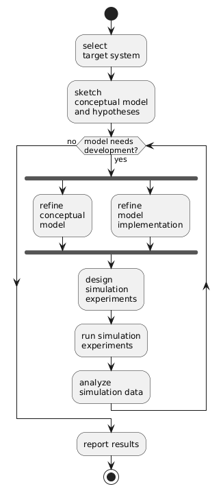
Figure f:modelingProcess provides a stylized illustration of key steps in model development and analysis. [1] Scientific model development typically involves hypothesis generation, experimentation, and data analysis. This book correspondingly shows how to run simulation experiments, to analyze the resulting data, and to report the experimental results.
Stylized Simulation Modeling Process
Many social science models can be investigated without computational tools, and this is true of the model of the present chapter. However, relatively simple computational models can often solve problems that are mathematically challenging or even intractable [Humphreys-2002-PhilSci]. This is particularly true of dynamical models. As shown in subsequent chapters, computational models facilitate the investigation of the complex dynamics that can emerge even in apparently simple models.
Conceptual Models and Their Implementations
Scientists often build models in order to explore how a target system behaves. Model development often begins with a somewhat vague and incomplete conceptual model. This conceptual model is typically descriptive. It might be verbal, diagrammatic, or even mathematical, but it is not implemented in a programming language. This book demonstrates how to transform conceptual models into computational models. A central goal of each chapter is to implement a conceptual model as a computational model, in order to simulate the behavior of a target system.
A computational implementation produces a computational model of the system, which is an algorithmic implementation of a conceptual model that is executable on some kind of computer. Modern simulations typically run on electronic digital computers. There is a natural give and take between conceptual models and computational models. Concepts drive computational modeling, and the process of computational modeling can lead to improvements in the conceptual model. In Figure f:modelingProcess, refinement of the conceptual model and of the implementation take place in parallel, making use of the results of previous refinements.
Running a computational model on a computer produces a simulation of the target system. A dynamical simulation explores the evolution of a system over time. One goal of simulation is to generate insights into the behavior of the target system. Some simulations are purely playful explorations. More often, the purpose of a simulation experiment is to gain insight into the behavior of a real world dynamical system.
Why Use Simulation?
Key competitors to simulation modeling are narrative modeling and mathematical modeling. Narrative modeling is the verbal presentation and analysis of a conceptual model. Mathematical modeling is the mathematical presentation and analysis of a conceptual model. Each has its strengths and weaknesses; there is no best approach to modeling. The choice must be pragmatic, considering the appropriateness of each approach to the problem at hand.
As a key consideration, simulation modeling often enables the incorporation of salient details that might bedevil mathematical modelers while avoiding the lack of rigor that may bedevil narrative modelers. Cost effectiveness is another key consideration. The applied physical sciences often use simulation to produce speedier and cheaper investigations of target systems. Practically, simulations can be the most cost effective means to rigorously investigate the behavior of a physical system.
Simulation modeling has fruitfully elucidated many real-world systems, including applications in science, engineering, and business. An example from physical science would be simulations of the interplay of molecular forces during protein folding. An important example from medicine arises in the drug discovery process, which involves simulating the interaction between chemical compounds and biological targets. An example from engineering would be simulations of airflow over different wing designs to detect effect on lift and control. An example from business would be simulations of how supply chains affect the reliability of product distribution.
This book emphasizes social-science applications of modeling and simulation. We may also be interested in responses of systems to variables that we cannot ethically manipulate, including environmental variables that affect human safety. Narrative and mathematical modeling can share with simulation modeling the ability to conduct experiments that would be infeasible or unethical to attempt in the real world. However, simulations are often be the only practicable means of rigorous investigation. For example, it is infeasible to design a large-scale evacuation plan by deliberately experimenting with large-scale evacuations in the real world. A narrative approach to this problem will lack needed rigor, while a purely mathematical approach may prove intractable. Simulation may allow a cost-effective comparison of different evacuation plans.
System Dynamics
stock variables and flow variables
physical implementations vs software implementations
discrete-time dynamical systems
system state
evolution rule
function iteration.
A dynamical system evolves over time. A model of a dynamical system characterizes this evolution. Abstractly, a dynamical model must characterize every possible state of the system and provide an evolution rule for the system. The evolution rule describes how the system moves from one system state to another. Given an initial system state, the evolution rule determines how the system state evolves over time. Together, the evolution rule and the initial system state determine the trajectory of the system.
Modeling Dynamical Systems
System dynamics and agent-based modeling are two prominent yet divergent approaches to the computational modeling and simulation of evolving systems. Both approaches have proved their worth for social scientists. This book focuses on the agent-based approach, but this chapter and the next provide a brief introduction to the system-dynamics approach. This introduction emphasizes a basic structure of simulation modeling that both approaches share.
Stocks and Flows
stock variable: measurement at any point in time
flow variable: measurement refers to a period of time
The system-dynamics approach to social-science modeling and simulation gained popularity in the 1950s. In system-dynamics models, aggregate outcomes result from the dynamic interplay of aggregate quantities. The model dynamics result from the interplay of aggregative stock variables and flow variables.
A flow variable represents a rate of change. Flow variables must be defined with respect to a period of time, using a specific time unit. In contrast, a stock variable is defined at any point of time, without reference to a time unit.
For example, in a model of human disease transmission, the stock variables might include the number of susceptible individuals, the number of infected and infectious individuals, and the number recovered and immune individuals. The magnitudes of these variables can be measured at any point in time without reference to the passage of time. The rates of change of these stocks are flow variables, which must reference a (real or virtual) period of time. As another example, the total population is a stock variable in a simple model of population growth, while the annual rate of population growth is a flow variable.
A system-dynamics model characterizes how the overall behavior of a system is determined by the feedback between the stocks and flows in the system. In an infectious disease model, if the number of infectious individuals and the number of susceptible individuals are both large, then we expect a high rate of flow from the susceptible group to the infectious group. In a population growth model, there may be feedback from the level of the population to the size of its change. Dynamic interactions between the stocks and flows determine the evolution of the system.
Mathematical versus Computational Implementations
A system-dynamics model is typically implemented as a collection of computational functions that characterize these stock-flow interactions. However, other implementations are possible. For example, very simple models are amenable to exact mathematical solution. The population model of this chapter is in this class. Such models are pedagogically useful, since the exact correspondence between the mathematical model and the simulation model permits an easy comparison between the simulation results and the mathematical solution. This provides helpful guidance to simulation novices, who can readily check the validity of their computational implementation.
MONIAC
Demonstration videos:
Among economists, a particularly famous system-dynamics model is the MONIAC. The name is considered an acronym for monetary national income analogue computer. The MONIAC is an early computational implementation of a macroeconomic model, but it did not run on an electronic computer. Instead, the original implementation used a special-purpose hydro-mechanical analog computer. This physical implementation of the model is widely known as the Phillips Machine, after its creator. [2]
The MONIAC is very early example of a system-dynamics simulation model in the social sciences. It is a computational implementation of a macroeconomic model of the UK that was popular in the 1940s. Water levels represent stock variables (such as the money supply), and water flow rates represent flow variables (such as the rate of government expenditure). Phillips used this model to simulate the macroeconomic effects of changes in monetary and fiscal policy. The simulations also illustrated the importance of coordinating monetary and fiscal policy. These simulations were fundamentally dynamical: hydrological interactions evolved over time, and the full effects of policy changes emerged gradually.
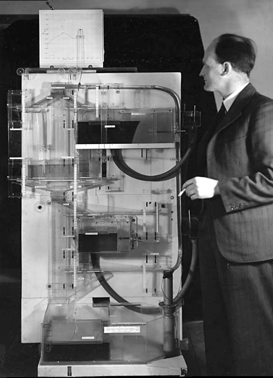
Bill Phillips with a MONIAC
Source: LSE Library
Methodological Differences: Aggregation
As subsequent chapters demonstrate, the macrostate in an agent-based model emerges from the interactions of many individual agents. System-dynamics models adopt a fundamentally different methodological approach: they rely heavily on the interactions between aggregates. For example, the MONIAC is a purely aggregative model. It produces aggregate macroeconomic outcomes (such as GDP) through the interaction of macroeconomic aggregates (such as total consumption). Individual agents are nowhere to be found in the model implementation, even if they are implicit in the underlying conceptual model.
Implementation Differences
The most striking difference of the MONIAC from contemporary simulation methods is its physical implementation. Nowadays, system-dynamics models are typically implemented in software in order to run simulations on a digital computer. A typical implementation of a system-dynamics model comprises a set of computational functions. The computer executes these functions in order to simulate the dynamic behavior of a system.
This difference is not conceptually fundamental. Nevertheless, it is practically important, because physical models are costly and time-consuming to build (and to run). Implementing the same computational model on a modern digital computer, using a modern computer programming language, results in substantially lower costs. Indeed, for a while the Reserve Bank of New Zealand website featured a MONIAC implemented in software.
Discrete-Time Modeling and Simulation
The hydrological MONIAC implemented a continuous-time dynamical system. In this model, time moves continuously as water flows between physical chambers. In contrast, the population model of the present chapter characterizes the system only at discrete points in time. It is a discrete-time dynamical system: time in the model progresses in discrete increments. A single increment is often called a step, model step, time step, period, or tick.
The conceptual temporal size of a model step is the time scale of the model. The real-world temporal interpretation of a time step is model-specific; an increment can be as crude or refined the target system requires. For example, one time step in a simulation model may represent a conceptual hour, day, month, or year. In the population growth model of this chapter, a single model step represents one year.
State Transition
At time \(t\), a discrete-time dynamical system is in some state. Call it \(s_t\). For example, in a population growth model, this might be the current level of the population. By applying the evolution rule of the system, it transitions to another state, say \(s_{t+1}\). Given an initial system state, repeated application of the evolution rule produces future system states.
Abstractly, the evolution of a computational model from its current state to the next state is governed by a function. This is the evolution rule or state-transition function. In the discrete-time simulation models of this book, the current model state directly determines the subsequent model state. Letting \(s_t\) represent the model state at time \(t\), and letting \(f\) represent the state-transition function, adjacent states are related by the equality \(s_{t+1} = f[s_{t}]\). [3]
Function Iteration and the State Trajectory
Iteration is the repetition of action. Function iteration is the repeated application of a function to produce a sequence of values. (See the Glossary for more details.) For example, starting from an initial state of \(s_0\), repeatedly apply the evolution rule \(f\) to produce the following iterates of \(f\).
That is, given an evolution function (\(f\)) and an initial state (\(s_0\)), function iteration generates the implied state trajectory of this model. Here the state trajectory is the sequence \([s_0, s_1, s_2, s_3, \ldots]\). As a convenient mathematical notation, write \(f^{\circ n}[s_0]\) to denote the result of iteratively applying the function \(f\) a total of \(n\) times, given the initial value \(s_0\). Then we may summarize all of these equations as follows.
The population model of this chapter iteratively applies a basic exponential-growth rule. Given an annual growth rate and the current population, the model determines the population trajectory for subsequent years. Later chapters consider models where the only feasible representation of the state transition function is the actual computational implementation of the entire model. However, a very simple model may imply an easily understood mathematical representation of the state-transition function. As shown in the next section, the population growth model of this chapter serves as an example of such simplicity.
Mathematical and Computational Functions
mathematical vs computational functions (pure & impure)
command-line tests
the concept of a computational activity
introduction to testing
As illustrated by Figure f:functionBlockDiagram, it is often convenient to think of a mathematical function as a rule for transforming inputs into outputs. From this perspective, a univariate real function accepts a real number as an input and produces a real number as an output. For example, a squaring function transforms a number into its square by multiplying the number by itself. This conceptualization of functions as transformation rules applies as well to computational functions, which provide a way to perform such transformations on a computer.
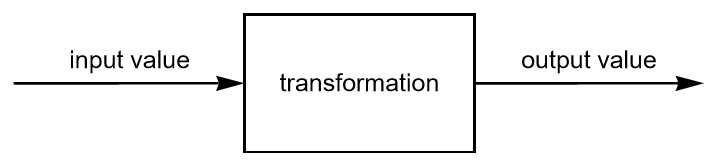
Block Diagram for an Abstract Function
What is a Function?
Consider transforming a number by multiplying it by \(1.01\). This is a very specific example of a univariate real function. A typical mathematical expression of this function is \(x \mapsto (1 + 0.01) * x\). (The term map is a synonym for function, and we pronounce the \(\mapsto\) arrow as maps to.) This representation of the function simply states its transformation rule. At this point, the function does not have a name.
Applying this specific function to an input value of \(100.0\) produces an output value of \(101.0\). For such a simple calculation, we do not even need a computer. Nevertheless, as shown below, this function can represent behavior in a system of interest. Specifically, interpret this function as the yearly evolution rule for the world population. Under this interpretation, the function characterizes the evolution of the population in a world that has a fixed annual population growth rate of one percent.
Function Parameters in Mathematics and Computations
mathematically, distinguish bound variables vs. free variables
computationally, distinguish local variables vs global variables
The expression \(x \mapsto (1 + 0.01)*x\)
represents a function by specifying its transformation rule.
Note how this expression uses a variable named x
to abstract refer to any particular input the function might receive.
This \(x\) is the function parameter.
In the function definition,
a parameter does not denote a particular value.
Instead, it represents any possible value that the function may be applied to.
Correspondingly, any other name serves just as well, as long as all occurrences in the function definition change in the same way. For example, the expression \(p \mapsto (1 + 0.01) * p\) represents exactly the same function. Mathematical discussions commonly use a single lowercase letter for the function parameter, but this is just a convention. For example, the expression \(\square \mapsto (1 + 0.01) * \square\) can represent exactly the same function.
These superficially different expressions represent the same function because they all describe the same relationship between inputs and outputs. Changing the parameter name does not change the meaning of the expression. The parameter is fundamentally a placeholder that makes it easier to understand the transformation of inputs into outputs. The name chosen to designate the input value does not affect how the function behaves. In fact, it has no meaning outside of a particular function definition.
Here is another way to say the same thing: a function’s parameters are bound by the function’s definition. This is true of both mathematical functions and computational functions. This means that the name chosen for a function parameter does not interact with the surrounding context, whether mathematical or computational. In fact, it has no meaning at all outside its particular function definition. So when naming a parameter, just choose a name that best aids a reader to understand the function.
From Mathematical to Computational Functions
This need to create computational functions is so common that almost all programming languages make it extremely simple to define computational functions. This allows computer programs to incorporate useful mathematical functionality by implementing mathematical functions as computational functions. For example, this section shows how to include the population growth function in a computer program.
Recall Figure f:functionBlockDiagram, which characterizes a function as a transformation of inputs into outputs. A particular input value to a computational function is the function argument, and the corresponding output value is the return value. Applying a computational function to an argument (of the right type) produces a return value.
What is a Pure Function?
A pure function is
closed
side-effect free
Many programming languages provide facilities for defining pure functions, which are the computational analogues of familiar mathematical functions. A pure function is closed and side-effect free. (See the Glossary for more details.) The definition of a pure function ensures that any given input value always produces the same output value.
A pure function is closed. A function whose output is determined solely by its explicit input is closed to other influences. Roughly speaking, when a computational function is closed, knowing just the value of its argument is sufficient to determine its return value. It does not depend on the context in which the function is executed. This makes it easier to understand how the function will behave whenever we use it.
A pure function is also side-effect free: executing it does not modify the environment in which it runs. Examples of environmental modification include changing the value of a nonlocal variable, writing data to a file, or communicating with a computer peripheral. This is often a desirable property, yet producing side effects is often desirable as well. Later sections return to this problem. Our first task, however, will be to implement a pure function.
Planning the Implementation
Good implementations sometimes require extensive planning. However, in a case as simple as this population growth function, very little planning is needed. Even so, it can be useful to sketch a basic function summary, if for no other reason than to nurture the habit.
A function summary may be extremely informal and sketchy,
or it may be quite formal and detailed.
The level of detail should reflect both
the immediate needs of the programmer
and the anticipated needs of possible future readers of the code
(i.e., anyone who might try to understand the code).
One common to detailed description is pseudocode,
which roughly resembles an implementation in a programming language,
Instead of pseudocode,
this book sketches functions (and other subroutines)
in a simple outline format.
Here is a function sketch for the population growth function,
named nextExponential01.
- function signature:
nextExponential01: Real -> Real- function expression:
\(p \mapsto 1.01 * p\)
- parameter:
\(p\), the population
- summary:
Grow the population by 1%.
Notation in Code Sketches
Code sketches in this book freely use simple mathematical notation,
which often resembles but need not match
the notation in any particular computational implementation.
For example, it is convenient to provide a very short name to represent an arbitrary input;
this is the function parameter (here, p).
A function sketch typically expresses
the output as an expression involving the function parameter
(here, \(1.01 * p\)).
In actual code, one may prefer a longer, more informative
parameter name (e.g., pop or even population).
Additionally, the function sketches in this book
usually state the data type of the valid inputs and of the return values.
The notation Real -> Real means that
the function maps a real-valued input to a real-valued output.
This specifies the input type and output type to both be Real,
which name the typical computational data type for representing real numbers.
(The exact meaning of this varies across programming languages.)
Create a project file for the PopulationGrowth01 project.
In the project file, implementing the nextExponential01 function,
following the code outline above.
Include helpful comments in your code,
and remember to save your model after changing it.
Define a pure function: it must not depend on any other code, and it return a deterministic numerical output when applied to any numerical input. It should have no side effects. (For example, it must not print.)
Testing of nextExponential01
A useful rule when programming is to presume that untested code is broken.
So, after creating the nextExponential01 function,
it is time to test it.
A first and simplest test is to apply this function to an
argument and then print the result,
in order to check that it behaves as expected.
It is a pure function, so it is particularly easy to test:
the correct output for any specified input is completely predictable.
Recall that nextExponential01 is a computational implementation of
the mathematical function \(p \mapsto (1 + 0.01) * p\).
One test of this implementation might apply the computational implementation of this function
to the value 0.0 and test that the return value is 0.0.
If the return value differs from 0.0,
the test must signal this failure in some way.
This book provides a very limited discussion of software testing,
focusing on simple and sometimes ad hoc tests.
Ad hoc testing by printing and then inspecting outputs
can initially prove useful, but it soon becomes tedious.
More automated testing is evidently desirable.
An automated test of a single component of a program,
such as a function, is often called a unit test.
The next exercise is to create a unit test for the nextExponential01 function.
First, try a little ad hoc testing.
The best way to do this is language dependent,
but to get started, do it interactively if possible.
Apply the nextExponential01 function to an argument of 100
and print the result. The result should equal 101.
Apply the nextExponential01 function to an argument of 1000
and print the result. The result should equal 1010.
Next, automate the previous test of the nextExponential01 function
by adding a unit test to the PopulationGrowth01 project.
Additionally, test that output is correct for at least the following inputs:
-100.0 and 0.0.
Exponential Population Growth and Discrete-Time Simulation
population dynamics
rates of change vs. growth rates.
exponential growth.
application: exponential population growth
describing the simulation structure.
initializing a simulation model.
defining a simulation schedule.
create data visualizations.
This section describes a computational implementation of the first population growth model. A preliminary discussion of the difference between rates of change and rates of growth provides background to the concept of exponential growth. After introducing a standard structure for discrete-time simulation modeling, the present section develops a simple discrete-time dynamical model of the world population. Running the model simulates population growth over time and produces forecasts of future population levels. (A subsequent chapter improves upon this oversimplified forecast.) The section concludes with a brief introduction to the visual display of simulation data.
World Population Growth
The empirical observation that motivates the exponential-growth model is the remarkable increase in the world population since the First Agricultural Revolution [BocquetAppel-2011-Science]. Figure f:HistoricalWorldPopulationLevels illustrates world population estimates over several thousand years. Clearly, human population growth has not been a linear function of the time passed.
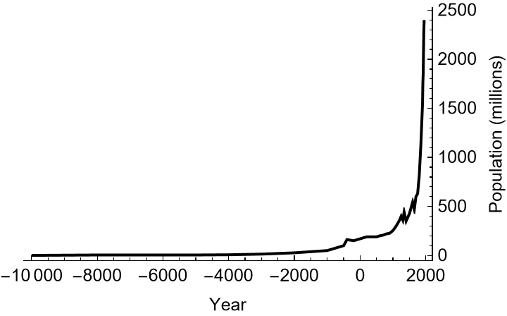
World Population Estimates (10000BCE–1950CE)
Data Source: United Stated Bureau of the Census
This section demonstrates that a particularly simple aggregative model can roughly mimic such growth. Modeling the world population as a single aggregate stock of people disregards individual-level attributes. For many social-science questions, a less aggregative approach is advantageous. Later chapters explore such disaggregation in detail. However, this chapter first illustrates some basic simulation tools by exploring a particularly simple system-dynamics model at the highest level of aggregation.
Rate of Change vs Growth Rate
Let the current world population (\(P_{t}\)) be the state of this system. Population is a stock variable: it can be measured at any point in time, without any reference to a period of time. The system state comprises this single stock variable. Since the world population can only assume nonnegative values, the possible states of the system correspondingly are nonnegative numbers.
The net addition to the population in a specified period is a flow variable. Abstractly, in a system dynamics model, flows affect stocks. Concretely, in the present model, the total population changes as a result of any net addition. The change in the population produces a change in the state of the system.
If \(P_t\) is the population at time \(t\), then \(P_{t+1}-P_{t}\) is the rate of change for the period from \(t\) to \(t+1\). Define the one-period growth rate from \(t\) to \(t+1\) to be the proportional rate of change over the period. (This is sometimes called the proportional growth rate.) Let \(g_{t,t+1}\) denote this growth rate, computed as follows.
For example, Figure populationLevelsGrowthUS illustrates historical population levels in the United States, along with the associated annual growth rates. Evidently, there can be substantial short-run variation around the mean growth rate even in a large country. For example, even though it is not particularly evident in the plot of the population levels, it is very easy to detect a post-WWII baby boom in the plot of the annual population growth rates.

US Population Levels and Annual Growth Rates
Data Source: FRED series B230RC0A052NBEA.
Evolution Rule for Exponential Growth
Real-world population growth is a complicated process, difficult to model and to accurately predict. Numerous real-world factors continually impinge upon population growth rates and should therefore be incorporated into demographic projections. Nevertheless, as an initial introduction to population growth, this chapter focuses entirely on a particularly simple special case. To support the development of both conceptual understanding and modeling skills, assume the population grows at a constant rate (\(g\)). The implies that the population at adjust periods is related as follows.
This is the evolution rule for the population. It states that there is a simple dependence of next period’s population on the current population. In this simple dynamical system, the evolution rule implies exponential growth at a constant rate \(g\).
A discrete-time population growth model describes how the population changes from period to period (e.g., from year to year). The population \(P_{t}\) constitutes the system state at time \(t\). A state trajectory for this model is a sequence of populations over time. From any given initial population, repeatedly applying the evolution rule produces projections of future populations. Concretely, given a growth rate \(g\) and an initial population \(P_0\), compute the population \(P_t\) by iteratively (i.e., repeatedly) multiplying by \((1+g)\). Here are the first three iterations.
This population model is so simple that a mathematical solution is ready at hand. The model implies an interesting, useful, and particularly simple mathematical relation, which concisely characterizes the population at any time \(t\).
From Mathematics to Simulation
It is evident from the mathematical solution that even a simple calculator can quickly produce a population projection for any desired year. In this sense, there is no substantive need to simulate the evolution of the system. However, the very simplicity of the model implies a pedagogical utility in implementing it. The availability of a mathematical solution makes it simple to test simulation results for accuracy. Furthermore, the implementation will elucidate a simulation process that applies to more complex systems. As later chapters demonstrate, many dynamical systems that are nevertheless tractable for simulation lack a simple mathematical solution.
Beginning with a conceptual model of the dynamical system, simulation modeling begins by implementing a matching computer simulation model. Executing the resulting code is called running the simulation. This simulates the evolution of the system over time. Running the simulation typically involves iterating the computationally implemented evolution function for the system. Computers are excellent tools for repetitive tasks. The computer instructions for performing any action once provides the basis for performing the same action repeatedly. When modeling a discrete-time dynamical system, looping constructs allow easy iteration of the evolution rule.
High-Level Simulation Structure
Figure f:runsim01 outlines this typical simulation structure of a discrete-time simulation. It shows , an initial setup phase followed by the iteration phase. The iteration phase repeatedly executes the model schedule, until a stopping criterion is satisfied. Each execution of this schedule is called a model iteration or a simulation step. Crucially, this simulation schedule embodies the evolution rule for the model. Later chapters add a wrap-up phase, comprising activities to perform after the iteration phase is complete.
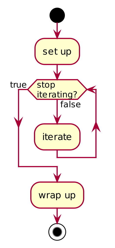
Stylized Discrete-Time Simulation
Parameters of the Simulation Model
In order to produce population projections, the exponential growth model requires only an initial population and a population growth rate. These are the model parameters; they should not change as a simulation runs. An implementation of a numerical population simulation needs to provide numerical values for the model parameters. Table t:ExpGrowPrms suggests possible parameter values.
name |
value |
meaning |
|---|---|---|
|
8.25 |
initial population (in billions) |
|
0.01 |
constant annual growth rate |
Our nextExponential01 function
hard codes the growth rate parameter.
That is, it includes the population growth rate
of 1% literally in the function definition.
Although hard coding is a rather brittle approach to parameterization,
retain this implementation for now.
An often preferable alternative to hard coding is to
introduce model parameters as named global constants.
Global Constants
As an example of a named model parameter,
let pop0 denote the initial population level.
Assume this name has has global scope,
which roughly means that any portion of a model’s code can refer to it.
Equivalently, the name pop0 will be visible everywhere
in the PopulationGrowth01 model.
Problematically, in some languages
this means that any portion of a model’s code can potentially change its value.
When a programmer cannot enforce constancy of a global value, one part of the model code might change a value that another part expects to be unchanged. Keeping track of such expectations can be difficult. For this reason, programmers should only reluctantly introduce global variables and must always handle them carefully. Despite this brittleness, the use of global variables can simplify early model development, and this book introduces them rather freely. The payoff is often easier to read example code, from which the global variables subsequently can be purged by more experienced readers.
Some languages include features for enforcing parameter constancy; others leave it up to the care of the programmer. In either case, running a simulation should not change any model parameter. Although neither hard coding nor the use of global constants is a particularly good approach to parameterization, both are quite commonly used in simulation modeling. (A subsequent chapter explores alternatives.)
Initializing the Model Parameters
A simulation requires initialization of the
model parameters before it can run.
Parameter initialization is part the setup phase of the model.
For the PopulationGrowth01 project,
initialization is trivial:
just set the value of pop0 (the initial world population).
Add pop0 as a parameter of the PopulationGrowth01 model.
Test that you can apply nextExponential01 to this parameter
and produce the expected value.
Iteration Phase
At a high level of abstraction,
running this population growth simulation may be divided into two main phases:
a setup phase, and an iteration phase.
The setup phase comprises preparations to iterate a simulation schedule,
including setting up the initial model state (here, the initial population).
The iteration phase repeatedly executes the simulation schedule,
which repeatedly updates the model state (here, the total population).
Each simulation step updates the world population:
it applies the nextExponential01 function
to the previous population projection in order to produce the next population projection.
This is the core of the iteration phase of this population simulation:
repeatedly executing the simulation schedule until the simulation terminates.
Our stopping criterion will be arbitrary:
we will produce \(50\) annual population projections.
While researchers sometimes care only about the final state achieved by a simulation,
it is more common to track the evolution of the simulation over time.
Tracking requires collecting simulation data at regular intervals,
perhaps at the end of each iteration.
The sequence of collected data is the output trajectory for the simulation.
For example, population modelers often produce annual projections
for a prescribed number of decades into the future.
These projections derive from the output trajectories produced by their simulations.
The following sketch of a printTrajectory activity_ encompasses
the setup and iteration phases for the current population model.
- activity name:
printTrajectory- summary:
Set up the simulation, as needed.
Starting with the initial population stored in
pop0, iterate the simulation schedule a total of50times to produce the 50 annual population projections.Print the trajectory (i.e., the initial population along with the 50 population projections).
During the iteration phase, a common need is to gather data from the simulation. There are many ways to do this, which later chapters explore in detail. For now, simply print the simulation values. However, the activity sketch is somewhat loosely formulated to allow some reader freedom. In particular, it does not say whether population projections are printed as they are produced or all at once after they have all been produced. In either case, the simulation produces \(50\) iterations of the simulation schedule.
Imagine that you are a demographer.
Use your knowledge of the current world population (look it up)
while asssuming a constant future population growth rate of 1% per year.
Simulate an annual population trajectory over the next \(50\) years
by following the activity sketch above.
(Add a printTrajectory activity to the PopulationGrowth01 project.)
The setup phase should fully prepare for the iteration phase,
which should iterate the nextEponential01 function.
(Use any iteration method you choose.)
Display the projections any way you wish (e.g., simply print them).
Procedural Approach:
Create a printTrajectory procedure or other subroutine
that runs the entire population simulation and prints the resulting trajectory.
Alternative Approach:
Create a trajectory function that returns
a sequence (such as a list or array)
that contains all of the population projections.
Print this trajectory.
Stretch Exercise:
Refactor the trajectory function so that it requires three arguments:
the initial population, the growth rate, and the number of iterations.
The Need for Data Visualization
Up to now, the only access to the simulated population trajectory has been through a visual examination of printed numbers (i.e., the population forecasts). This is far from adequate: these printed results typically provide very limited insight into the simulation outcomes. Later chapters explore a variety of tools for improving our understanding of such data. Data-visualization tools will play a particularly important role. Data visualizations may expose patterns in the evolution of a simulation or in its final outcomes that might otherwise be missed.
A normal human eye can process a remarkable amount of visual information very quickly, often detecting even faint patterns or small anomalies with ease. Charts displaying the generated data can therefore promote understanding of the simulation outcomes. Of course, humans are subject to perceptual illusions and limitations: we may detect patterns where there are none or miss patterns that exist. Nevertheless, visual representations of simulation output often prove indispensable.
Run-Sequence Plots
This section concludes with a univariate visualization that has long been in wide use: the run-sequence plot. A basic run-sequence plot consecutively displays a single sequence of values, ordered by their locations in the sequence. For the current project, this will be the population projections for each year.
Many simulation toolkits and even many programming languages offer extensive facilities for data visualization. The available plotting facilities vary widely across languages, and the ease of use of these facilities varies considerably. In some languages the readily available plotting facilities are so limited that it typically pays to export the data to a file for input into a separate plotting program. [4] Future chapters explore data export in some detail.
Population-Projection Plots
Static plots are often fully adequate to the analysis of simulation output. Even so, creating an attractive and communicative plot can be challenging. For example, patterns in the underlying data may be exposed or hidden by something as simple as the axes ranges or scaling.
It sometimes proves useful to draw the recorded model states as an animated plot. In some cases, this may better communicate the evolution of the model state. In addition, simulation toolkits often take an additional step and support dynamic simulation plots. An animated plot is dynamic if it is repeatedly redrawn as the running simulation model provides new updates of the model state. This can be particularly useful for monitoring longer running simulations.
The best approach to plotting is highly toolkit specific. Some languages and simulation toolkits support easy GUI building that includes facilities for simple plot construction and display. Others require substantial additional code even for simple static plots. Regardless, plot creation generally has two components: setting up the options for the plot window, and plotting the data. Important plot options typically include the numerical limits of the two axes and an informative choice of axes labels.
- activity name:
plotTrajectory- summary:
Set up the simulation, as needed.
Starting with the initial population stored in
pop0, iterate the simulation schedule a total of50times to produce the 50 annual population projections.Plot the trajectory (i.e., the initial population along with the 50 population projections).
Implement the plotTrajectory activity.
Simplest Approach: Copy printed population projections into a spreadsheet and make a line chart.
Better Approach: If supported by your chosen simulation toolkit or programming language, add to this project the creation a line chart of the population projections.
Stretch Exercise: Create an animated (possibly dynamic) run-sequence plot of the population projections. For this exercise, plot updates should be sequential, repeatedly adding a single point to the plot.
Sample Population-Projection Plot
Figure f:exponentialGrowthPlot provides an example of a chart based on the data generated by this population model. The smooth upward trend in the population is readily apparent, as is the increasing slope of the population trajectory. The ease with which we discover these features in the data demonstrates the analytical utility of data visualizations. Plots can make it easy to detect data behaviors that are hard to detect in printed output.
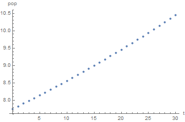
Population Projections (Exponential Growth)
Summary and Conclusions
This chapter introduces the process of modeling and simulation, with an emphasis on discrete-time system dynamics. At the core of system dynamics is the interaction between stock variables and flow variables, each as an aggregative concept (such as an entire population). The present chapter highlighted the effect of a flow on a stock, but subsequent chapters emphasize two-way interactions. System dynamics modeling typically uses functions to summarizes these aggregate interactions. Correspondingly, this chapter spends some time exploring the relationship between mathematical and computational functions.
In the terminology of this book, a computational function transforms inputs into outputs. A pure function ensures that a given input always produces the same output, with no other side effects. In the terminology of this book, an activity_ is a computational subroutine that does not return a value but instead produces changes in the program environment (including all kinds of program output). In a procedural language, such an activity may be handled by a named procedure, which in turn makes use of functions.
This chapter develops a simple population simulation,
where population growth is exponential at a constant rate.
The implementation iteratively applies the nextExponential01 function
in order to produce a sequence of population projections.
Such function iteration lies at the conceptual core of discrete-time simulation modeling.
This chapter also explores the relationship between a conceptual model and its computational implementation. An underlying conceptual model of population growth engenders a simple computational model. In order to practice decomposition—breaking models into simple, reusable pieces—this chapter follows a stepwise implementation of the simulation model. There is also a brief discussion of testing, in order to promote the development of correct and maintainable code.
This chapter concludes with a brief introduction to data visualization. Plots that facilitate data analysis need not be difficult to produce, as illustrated by a run-sequence line chart of the population projections. The line chart in Figure f:exponentialGrowthPlot uses data generated by this simulation model of population growth.
Note that despite the 50 year forecast horizon, the nonlinearity of exponential population growth is only slightly visible in Figure f:exponentialGrowthPlot. Extending the population projections further into the future augments the perception of nonlinearity. This is because a 1% growth rate of population produces doubling approximately every \(70\) years. It follows that if the \(50\) year projections perhaps appear shocking, projections over \(150\) years will appear utterly impossible. This implausibility motivates the model changes of the next chapter, which drops the assumption of a constant rate of population growth.
Exploration, Resources, and References
Supplementary Exploration
Helpful code comments are a good coding practice. Comments can specify the meaning of each model parameter or global variable. In some languages, comments can be useful for expressing the intended type of each variable. For example, a comment can specify that a variable should always have an
Integertype. This is useful when the implementation language does not support explicit typing of variables. Add such comments to thePopulationGrowth01project.Discrete-time simulations often include a global measure of time elapsed (i.e., the number of iterations). Conventionally this is often named
ticks. Add aticksvariable to the population model, initializing it to0and incrementing it near the end of each iteration. Thisticksvariable is inessential: it simply tracks virtual time in our simulation. In this population simulation, one tick will represent the passage of one year. This is the time-scale of the simulation model.Allow the growth rate each period to be subject to a transient random shock. How does this affect your population simulations? Allow the growth rate each period to be subject to a persistent random shock. How does this affect your population simulations?
(Advanced) Export the simulation data and use a spreadsheet (or other plotting software) to plot your population projections.
(Advanced) Instead of hard coding the population growth rate, make it a model parameter (say,
gE). Control its value with a slider in the model’s GUI.
Additional Resources
Function Iteration
Readers wanting a refresher for basic mathematical concepts may find [Feldman-2012-OxfordUP] particularly accessible and helpful. See chapter 1 for an elementary review of functions. Chapters 2 and 5 provide a brief, elementary overview of the concept of function iteration. The Wikipedia entry on iterated functions is also a useful resource.
Methodology
[Frigg.Nguyen-2016-Monist] provide a probing discussion of the relationship between models and their target systems, complete with useful examples and many helpful references. Also see [Swoyer-1991-Synthese], whose broader notion of surrogative reasoning links to the suggestion in this chapter that researchers experiment with models in order to learn about the target systems.
Testing
As a crude rule of thumb, never assume that untested code works as intended. Accordingly, computational models typically include tests, which help ensure that the code is working as intended. Some programming languages include extensive facilities for testing. Software testing is a huge topic that the present book treats in a cursory manner. Among the many excellent books and articles on how to test and maintain computer software, [Myers-2012-Wiley] and [Jorgensen-2014-CRC] provide good introductions to serious software testing.
MONIAC
For additional historical details about the MONIAC, see [Bissell-2007-IEEECS]. [Ng.Wright-2007-RBNZB], and Phillips’s early published description [Phillips-1950-Economica]. In addition, Part II of [Leeson-2000-CambridgeUP] is devoted to the MONIAC. [Colander-2011-EconomiaPolitica] draws lessons from the MONIAC for contemporary macromodeling efforts. [Ryder.Cavana_Cavana.etal-2021-Springer] provide a detailed exploration of how to translate knowledge of the MONIAC into a modern system-dynamics formulation.
Currently a number of web videos of the MONIAC are available on the Internet. One of them is Making Money Flow, created by the Reserve Bank of New Zealand using its still-working MONIAC. A more extended demonstration is offered by the University of Cambridge. A wonderful bit of MONIAC history is provided by Tim Harford’s lecture on Bill Phillips.
Data Visualization
Interest in sophisticated data visualization has exploded since the computer revolution. However, data visualization has a storied history. [Friendly-2008chII1-Springer] provides an accessible and fascinating overview of the early history. [Tufte-2001-GraphicsPress] provides inimitable aesthetic guidance. The field is now so fast moving that moving that every year brings new developments. Even so, learning to make communicative charts using a spreadsheet or a simple plotting package such as Gnuplot remains a great starting point.
References
Bissell, Chris. (2007) The Moniac: A Hydromechanical Analog Computer of the 1950s. IEEE Control Systems 27, 69--74.
Bocquet-Appel, Jean-Pierre. (2011) When the World's Population Took Off: The Springboard of the Neolithic Demographic Transition. Science 333, 560--561. https://science.sciencemag.org/content/333/6042/560
Colander, David. (2011) The MONIAC, Modeling, and Macroeconomics. Economia Politica: Journal of Analytical and Institutional Economics , 63--82.
Feldman, David P. (2012) Chaos and Fractals: An Elementary Introduction. : Oxford University Press.
Friendly, Michael. (2008) "A Brief History of Data Visualization". In Chen, C. and H"ardle, W. and Unwin, A. (Eds.) Handbook of Data Visualization, Berlin, Heidelberg: Springer-Verlag.
Frigg, Roman, and James Nguyen. (2016) The Fiction View of Models Reloaded. The Monist 99, 225--242. http://dx.doi.org/10.1093/monist/onw002
Humphreys, Paul. (2002) Computational Models. Philosophy of Science 69, S1--S11. www.jstor.org/stable/10.1086/341763
Jorgensen, Paul. (2014) Software Testing: A Craftsman's Approach. Boca Raton, Florida: CRC Press.
Leeson, Robert. () AWH Phillips: Collected Works in Contemporary Perspective. : Cambridge University Press.
Myers, Glenford J. (2012) The Art of Software Testing. Hoboken, N.J: John Wiley and Sons.
Ng, Tim, and Matthew Wright. (2007) Introducing the MONIAC: An Early and Innovative Economic Model. Reserve Bank Bulletin 70, 46--52. https://www.rbnz.govt.nz/research-and-publications/reserve-bank-bulletin/2007/rbb2007-70-04-04
Phillips, A. W. (1950) Mechanical Models in Economic Dynamics. Economica 17, 283--305. http://www.jstor.org/stable/2549721
Ryder, William H., and Robert Y. Cavana. (2021) A System Dynamics Translation of the Phillips Machine. In: Feedback Economics: Economic Modeling with System Dynamics, 97--134. Cham: Springer International Publishing. https://doi.org/10.1007/978-3-030-67190-7_5
Swoyer, C. (1991) Structural Representation and Surrogative Reasoning. Synthese 87, 449--508.
Tufte, Edward R. (2001) The Visual Display of Quantitative Information. Cheshire, CT: Graphics Press.
Appendix: Exponential Growth (Implementation Details)
Implementing the Population Growth Project in NetLogo
This section provides guidance for an
implementation of the PopulationGrowth01 project
in the NetLogo programming language.
Beginning the Exponential Growth Project in NetLogo
A basic NetLogo model includes code, documentation,
and model-specific GUI components.
Nevertheless, a simple NetLogo project may be stored in a single NetLogo model file.
Based on your reading in the Introduction to NetLogo supplement,
launch NetLogo as save an empty model file as PopulationGrowth01.nlogo.
(You can keep all of your NetLogo files for this book in a single folder.)
Implementing nextExponential01 (NetLogo Specifics)
The first exercise is to add a nextExponential01 function to the project,
using the function details provided in the chapter text. [5]
The chapter says that this function transforms a real value into another real value.
Unlike most other programming languages,
NetLogo includes only a single numerical data type,
which is used to represent both real numbers and integers.
So you can largely ignore this detail.
As described in the Introduction to NetLogo supplement,
instead of saying that a function returns a value,
NetLogo programmers typically say that a reporter procedure reports a value.
The term reporter procedure refers to a computational function;
the value reported is its return value.
This terminology is NetLogo specific.
It reflects the fact that a reporter procedure uses
the report keyword to return a value. [6]
Reporter procedures cannot be defined at the NetLogo command line.
Therefore, add the code for a nextExponential01
reporter procedure to the Code tab of this project.
The following stub provides a simple outline of this exercise.
to-report nextExponential01 [#p]
  ;put the function definition body here
  ; (remember to `report` the result)
end
As discussed in the Introduction to NetLogo supplement,
the to-report and end keywords
begin and end the definition of a reporter procedure.
After the name of the function (nextExponential01)
comes a name in brackets (#p),
which is the function parameter.
Recall that a function parameter refers abstractly to any possible input to the function,
and be sure to use it in the function body.
Also recall that this book adopts the convention
of beginning the names of NetLogo function parameters with an octothorpe (#).
This is just a book-specific convention and is not required by the NetLogo language.
The body of your function definition must transform
the input argument and report the transformed value.
Do not forget to use the report keyword,
or your code will not compile.
It is good practice to add helpful comments to your code.
Recall from the Introduction to NetLogo supplement that
semicolon begins a comment that lasts until the end of the line.
Once added to the Code tab,
nextExponential01 is available globally to the project.
Not only is it available to the entire NetLogo program,
but it is also available at the NetLogo command line.
This enables easy ad hoc testing of the function.
For example, after adding this function to your project,
enter the following at the command line.
print (nextExponential01 100)
The print command prints a value to NetLogo’s output area.
If your function implementation is correct, it prints \(101\).
The parentheses around the function’s name and its argument
are entirely optional;
they are just a visual aid.
Note that the function argument is not delimited by parentheses or brackets. Contrast this to NetLogo’s definition syntax for reporter procedures. When defining a reporter procedure, the parameter names must be bracketed. When applying a reporter procedure to an argument, brackets around the argument are forbidden.
NetLogo programmers often use simple command procedures for unit testing.
Following the chapter exercise,
create a test-nextExponential test procedure.
Recall from the Introduction to NetLogo supplement that
a reporter procedure reports a value,
while a command procedure does not.
The definition of a command procedure
correspondingly begins with to instead of to-report.
Your test procedure should compare what nextExponential01
actually produces for an input to what you expect it to produce.
Remember that unlike many other programming languages
NetLogo uses the equals sign (=) for comparison,
not for assignment.
(This is also true of most spreadsheets,
Lisp dialects, and Logo dialects.)
Execute NetLogo’s error command if a test fails,
and provide a useful error message.
To illustrate, enter the following at the NetLogo command line.
if (nextExponential01 0.0 != 0) [error "bad result for 0.0"]
After adding your test procedure to the Code tab of PopulationGrowth01 project,
run it from the NetLogo command line (in the Interface tab).
If you run into difficulties while trying to create this test,
copy the following command procedure into the project’s Code tab
and then run it from the NetLogo command line.
If your nextExponential function is correctly implemented,
this test procedure prints that the test passed.
This particular test is written so that it executes error if a test fails.
This terminates the execution of the test procedure and displays an error message.
Global Constants (NetLogo Specifics)
Next, explicitly parameterize the initial population.
In NetLogo,
when model parameters are not simply hard coded,
they are rather commonly introduced as global variables.
Take that approach for pop0.
As discussed in the Introduction to NetLogo supplement,
a NetLogo project can declare global variables
at the top of the Code tab
by means of a single use of the globals keyword.
In contrast to some other languages, however,
NetLogo does not provide a simple way to freeze the value of a variable. [7]
Therefore, in NetLogo a global constant is no more than
a global variable that the programmer refrains from changing.
For now, declare pop0 as a global variable.
That is, make sure that globals [pop0]
occurs at the top of the model’s Code tab.
In contrast to some other languages,
NetLogo does not allow concomitant initialization of the value.
An idiomatic approach to initialization is to
create a setupGlobals procedure
whose sole task is to initialize the value of
any global variables.
This might seem a bit extravagant when we currently have just pop0
to initialize, but do it anyway to form the habit.
Add a setupGlobals procedure to the model’s Code tab.
This procedure constitutes part of the setup phase of the simulation.
Note that it has an important side effect:
it changes the value of a global variable.
Producing a Population Trajectory with NetLogo
The next exercise is to iterate nextExponential01
in order to produce \(50\) years of population projections.
Before attempting this exercise,
be sure to review the documentation of repeat
in the NetLogo Dictionary.
Additionally, review the
introduction to function iteration
in the Introduction to NetLogo supplement
and the
further discussion of function iteration
in the NetLogo Programming supplement.
While beginning to think about this exercise,
just work at the NetLogo the command line and
simply print the population after each iteration.
Use the let command to
introduce an initial population as a new local variable:
e.g., let pop pop0.
Change the value of the population variable with the set command.
Consider using NetLogo’s repeat command for iteration.
This approach simulates exponential population growth over time
and provides forecasts for the next \(50\) years.
To illustrate,
enter the following code at the NetLogo command line (not the Code tab)
to print population projections to the output area of the Command Center.
setupGlobals
let pop pop0 repeat 50 [set pop (nextExponential01 pop) print pop]
This work at the command line illustrates the printTrajectory activity.
To add such an activity to a NetLogo model,
we typically implement it as a command procedure.
Therefore, implement a printTrajectory procedure
that runs the entire simulation.
For the moment, data export will consist only of
printing each population projection when you compute it.
In this case,
the printTrajectory procedure is essentially just a wrapper
around the command-line approach shown above.
The printTrajectory procedure should
start with the setup phase,
which runs the setupGlobals procedure.
Then introduce a local pop variable that is initialized to pop0.
You can use a repeat loop to update pop 50 times,
printing the updated value each time.
When you are done, enter printTrajectory at the NetLogo command line.
This should print the same forecasts as before.
Recall that the Code tab of the PopulationGrowth01 project
should already contain the following code.
This must be in place before you can execute the printTrajectory procedure.
Although the globals declaration must come before any procedure definitions,
NetLogo does not care about the order in which procedures occur in the Code tab.
NetLogo automatically compiles all command procedures and reporter procedures
when it loads the model, so they are all immediately available to the entire model.
Run-sequence Population Plot in NetLogo
Wrap up the PopulationGrowth01 project
by creating a plot of the population projections.
Although it is possible to copy the projections from the Command Center
into a spreadsheet in order to plot this,
for the current exercise add plot creation to the project itself.
The NetLogo name denotes not just the programming language
but also the associated simulation toolkit.
The NetLogo toolkit makes it particularly easy to add GUI widgets
to NetLogo’s Interface tab.
Following the discussion of GUI elements in the Introduction to NetLogo supplement,
add a plot widget interactively in the Interface tab.
NetLogo makes dynamic plotting particularly simple,
so exploit that facility while completing this exercise.
First, review the discussion of NetLogo plotting in the Introduction to NetLogo supplement.
As discussed there,
add a plot widget via the Interface tab.
(Remember, adding a widget is not possible in the NetLogo Code tab.)
To add a plot widget,
right click where you want the plot,
pick Plot,
add a plot name (e.g., Population Projections),
set the axes limits,
and delete the example pen-update commands.
(Later projects explore some of the other options.)
Also, set the dropdown menu under view updates
in the Interface tab to the continuous option.
(Later projects discuss this option.)
Save your work.
NetLogo automatically creates a graphics window (or View) when starting up, which by default displays as a large black square. The current project makes no use of this window. If you wish, edit it to make it smaller, and then cover it with the plot widget to hide it altogether.
Finally, implement the plotTrajectory activity.
Create a plotTrajectory command procedure, of course,
but you may also wish to separate your plot setup code
(perhaps in a setupPlotEG procedure).
Regardless, in order to reset the plot widget before running the simulation,
the setup phase of the plotTrajectory procedure
should begin with NetLogo’s clear-all command.
To update the plot, the plotTrajectory procedure
can simply use plot pop (instead of the previous print pop).
Extending the First Population Model (NetLogo)
At this point you have completed the PopulationGrowth01 project in NetLogo.
If you also wish to attempt the chapter Explorations,
here are a few hints.
The NetLogo programming language does not support type annotations, but comments still provide guidance to readers of your code. Recall that NetLogo has a single numerical data type, used to represent both real numbers and integers. You may nevertheless want to indicate with a comment whenever you expect a number to take on only integer values.
As an unusual feature, NetLogo builds in a special
ticksglobal variable, which must be initialized with thereset-tickscommand. Use thetickcommand to increment the value ofticks.There are multiple ways to export plotted data. First, right-click a plot and choose
Exportfrom the context menu. Second, useexport-plotto export the data.See the Introduction to NetLogo supplement for an introduction to lists. Pay special attention to the discussion of
lput, which may be used repeatedly to grow a list that holds the population trajectory.
Implementing PopulationGrowth01 in Python
This section provides guidance for an
implementation of the PopulationGrowth01 project
in the Python programming language.
Beginning the Exponential Growth Project in Python
A simple simulation model can be placed in a single Python file.
This is a plain text file that holds the source code for the model.
For the PopulationGrowth01 project,
create a file named population_growth01.py.
This will be the project file,
which should include all of the project code and some basic documentation.
Implementing nextExponential01 (Python Specifics)
Next, add a nextExponential01 function to the project file.
The chapter provides a function sketch,
which specifies that this function transforms a real value into another real value.
In Python programs,
the float type provides the most common representation of
mathematical real numbers.
(See the discussion of
numbers
in the Python tutorial.)
This means the nextExponential01 function should accept
a floating point argument and return a floating point output.
Python offers two different ways to implement functions:
function literals (usually called lambda expressions),
and normal Python function definitions (defined with the def keyword).
The present project uses only normal function definitions.
For details, see the discussion of
defining functions
in the Python tutorial.
Note that function parameter names must be parenthesized in your definition.
Any subsequent code in the project file
can access the definition of nextExponential01.
(Python does not hoist function definitions.)
Another way to access this function is to import the project file as a module.
As a simple example, launch your operating system shell and
ensure that the current working directory is your project directory
(i.e., the folder that holds the project file).
Then enter the following at the shell’s command line.
.. code:: python
python3 -c "from population_growth01 import nextExponential01; print(nextExponential01(100.0))"
Here the -c switch instructs Python to execute the subsequent string as Python code.
So this command-line invocation applies the nextExponential01 function
to an argument of 100.0.
As always, a direct Python function call
uses parentheses to apply the function to a particular argument:
Python requires parentheses around the function’s argument.
The print function can print values to standard output.
Like any other Python function,
print also must be called with parentheses around its argument.
Continual testing is a critical part of code development.
If this command-line invocation produces correct output,
it constitutes a successful test of your implementation.
When applied to an argument of 100.0,
the nextExponential01 function
should return the value 101.0.
The command-line invocation above will fail if the code does not compile,
but it can also fail for other reasons.
As one way to test only compilability,
from the operating system’s command shell
enter python3 -m py_compile population_growth01.py.
This will raise an exception if the code fails to compile. [8]
Avoid adding new code to a project without discarding any old code that fails to compile.
(This rule becomes absolutely crucial when a group is developing code together.)
More generally,
test writing is a critical part of any project.
In Python, one may write test procedures that rely on
assert statements.
(Here the term procedure denotes any Python function with no explicit return value.)
For example, a correctly implemented nextExponential01 function
will pass the following simple test.
In order to run this particular test,
first copy the test procedure into the current project file.
Here are some alternative ways you may then run this test.
(The use of pytest is recommended.)
Start by launching operating system command shell,
and then change to the folder holding your project.
Imitate the command line invocation above (using the
-cswitch) to import and run this test.Launch Python’s interactive shell and enter the following at the Python prompt.
from population_growth01 import test_nextExponential01
test_nextExponential01()
Install the pytest package. From your command shell, enter:
python3 -m pytest population_growth01.py
If the nextEponential function is correctly implemented,
executing this test procedure produces no errors.
However, this particular test raises an AssertionError if
any component of the test fails.
This exception causes Python to halt execution and display an error message.
If your implementation fails this test,
compare it to the following code snippet,
which illustrates an implementation that passes the test.
The illustrative implementation declares and defines
a Python function named nextExponential01.
The name in parentheses (p) is reused in the function body
to refer to any input that a user might provide to the function.
That is, p is a function parameter.
The name p is arbitrary:
you could just as well use x or pop.
Function parameters are local to their function definition,
so they are isolated from the rest of the program code.
Global Constants (Python Specifics)
Next, explicitly parameterize the initial population.
In Python,
when model parameters are not simply hard coded,
they are sometimes introduced as global variables.
Take that approach for pop0.
Generally speaking, Python does not provide language facilities to enforce variable constancy. (The next chapter returns to this.) Enforcing constancy is fundamentally a responsibility of the programmer, who may simply initialize a global variable and then commit not to change its value. Once defined, a global variable is visible in its entire module (i.e., code file). Such global constants are typically defined at the top of a module, where a helpful comment may identify this intended constancy. (Take this approach for the current project.)
Some Python programmers follow a convention of capitalizing
global variables to help indicate they should remain constant.
While this book does not insist on that practice,
let us follow it for the present project.
Global variables can be simultaneously declared and intialized to any desired values.
At the top of the project file,
set the value of the initial population
(the model parameter POP0).
Producing a Population Trajectory with Python
The next exercise of the PopulationGrowth01 project
is to iterate nextExponential01
in order to produce \(50\) years of population projections.
Before attempting this exercise,
be sure to review the Python documentation of the for statement.
Command-Line Exponential Projection (Python Specifics)
You may produce your code wherever you find convenient: in a Jupyter notebook, an IDE, or in a text editor. However, while beginning to think about this exercise, let us work in the Python REPL, which is also called the Python command line or Python interactive shell.
Use the initial population and the growth rate from the chapter exercise.
Use the = operator to
introduce an initial population using a new local variable,
which will hold the population updates.
Use Python’s for statement for iteration.
For the moment, simply print the population after each iteration.
To illustrate, here is a simple approach to producing population projections
for the next \(50\) years.
Exponential Projection (Python Specifics)
It is possible to simply copy most of this simulation code
into the project file and then execute the file
to complete the printTrajectory activity.
Instead, let us refactor the code to produce a trajectory function,
which will return the entire trajectory as a
list.
This requires small changes in the approach above.
First, do not print as the simulation runs.
Instead, iteratively build a list from the population projections.
For example, start with the list [POP0]
and then append each new population projection to this list.
After the iteration phase is complete,
this trajectory function should return the entire list.
Here is one possible implementation.
The printTrajectory activity
runs the simulation and prints the results.
Ordinarily, we accomplish such an activity
by implementing and running a suitable procedure.
However, first try a command-line approach to this activity.
Using your operating system shell,
change to the project folder and
launch the Python interactive shell.
Then execute the printTrajectory activity
by entering the following code at the Python command prompt.
from population_growth01 import trajectory
print(trajectory())
Perhaps surprisingly, Python allows this.
There is no need for the user to provide a string representation of the list:
print function produces this automatically for any list.
As a slightly more interesting approach,
still from the Python command line,
print only one number per line.
It is possible to utilize a for statement to accomplish this,
iteratively printing each number.
However, with a little care,
Python’s print directly provides the needed functionality.
Use the asterisk splat operator to unpack the trajectory list,
and use the sep option to add a new line between each number.
Then execute the printTrajectory activity
by entering the following code at the Python command prompt.
print(*trajectory(), sep='\n')Run-sequence Population Plot (with Matplotlib)
Since printed values are of limited use in simulation modeling,
the final exercise in this project
is a plotting activity.
The goal is to create a visual display of the population trajectory.
Given the state of the PopulationGrowth01 project to this point,
a few alternatives for producing a run-sequence plot appear salient.
First and most crudely,
simply copy the printed data and paste them into a spreadsheet.
All modern spreadsheets allow easy line chart creation.
As a second alternative,
output the data to a file
and then use a plotting packgage (such as Gnuplot) to plot it.
(Subsequent chapters pursue this in more detail.)
A third and rather good option is to install a Python plotting package
and add the plotting code to the project file.
The following discussion chooses the third of these alternatives.
Plotting functionality is not built into Python.
Before attempting to plot the population trajectory,
we must install a plotting package.
One very popular and powerful Python plotting package is Matplotlib.
Install the package (e.g., with pip),
and then import it in the project file.
(See the discussion in the Basic Python Charts supplement.)
The following discussion relies on
the convenient pyplot interface.
Import this near the top of the project file (population_growth01.py)
by adding the following statement.
from matplotlib import pyplot as pltThere are many ways to build plots with matplotlib.
Most simply, a list named lst can be simply plotted
as plt.plot(lst).
A better solution does not simply rely on the default appearance,
but instead adds useful modifications—at the very least helpful axes labels.
How carefully to craft the plot details is a situation-specific decision,
depending on the purposes of the plot.
Given a decision to modify some plot details,
it may be helpful to isolate the plot-setup code.
In the following example code,
the setupPlotEG function provides a simple example.
This code explicitly accesses the figure and the axes for the plot
via Matplotlib’s subplots function.
This makes it very convenient to add a figure title
and axes labels.
Plotting the trajectory on the Matplotlib axis named ax
is as simple as ax.plot(trajectory).
This means that adding a plot
leaves the simulation essentially unchanged:
just replace printing the trajectory with plotting it.
However, keep in mind that Matplotlib does not display plots
until you request a display with the command plt.show().
The following example assembles all of these observations
into a plotEG procedure.
Finally, execute the plotTrajectory activity
by applying plotEG to the output of trajectory.
That is, simulate a population trajectory and then plot it.
from population_growth01 import trajectory, plotEG
plotEG(trajectory())
Extending the First Population Model (Python)
This completes the PopulationGrowth01 project in Python.
If you also wish to attempt the chapter Explorations,
here are a few hints.
Instead of using comments to indicate the type of each variable, use Python’s type annotations. Type annotations are not enforced at runtime, but a type checker (such as
mypy) can check them for consistency.Making
ticksa global variable (just for this project) may make it easier to check for implementation errors.Use Python’s
randommodel to generate random shocks.Data export to an external file is covered in the next chapter.
Copyright © 2016–2025 Alan G. Isaac. All rights reserved.
- version:
2025-09-09