Design, Analysis, and Reporting of Simulation Experiments
“A simulation study is an experiment that needs to be designed.”
Overview and Objectives
Overview
This lecture provides an overview of the design, analysis, and reporting of simulation experiments (DARSE). To be informative, an experiment must be well-designed, thoroughly analyzed, and adequately reported. Applications of experimental design and analysis range far beyond simulation modeling. This lecture considers a subset of issues that are immediately relevant to agent-based modeling and simulation (ABMS). Design considerations meld with analysis and reporting considerations, since a good experimental design is influenced by the anticipated analysis and reporting.
Goals and Outcomes
This lecture provides a brief introduction to the design of simulation experiments, approaches to their analysis, and some considerations in the reporting of results. In a broad sense, every lecture has considered in DARSE activities since the beginning of this course. However, this lecture introduces a more focused framework for these activities. To illustrates how DARSE increases the informativeness of simulation experiments, this lecture applies it to the Schelling segregation model.
Prerequisites
Establishing a Baseline
We build simulations as part of a search for useful models of a complex process. These simulations can prove useful in a variety of ways, from the improvement of understanding to the prediction or even control of real-world outcomes. This course emphasizes simulation models that produce new social-science insights, while also emphasizing the development of core simulation skills.
Baseline Description
Simulation results must be reported in the context of an implemented simulation model. Previous lectures illustrate approaches to model description, including the use of UML diagrams and variations on the ODD protocol. These approach to model description also guide the design of experiments.
This course approaches results reporting relative to a baseline. This includes a full description of the baseline parameterization, which is sometimes called the reference parameterization. It is a lucky simulation researcher who encounters a natural baseline. Often the choice of baseline parameterization will be somewhat arbitrary.
Baseline Parameterization
When a model’s parameters are clearly related to measurable real-world phenomena, researchers may choose baseline parameters from the existing empirical literature (or possibly original measurements). This is common in agent-based ecological models, but it is much less common in computational social science (with the partial exception of epidemiology). Social-science models are often marshaled to make a qualitative conceptual point rather than to enable quantitative prediction. The parameters of such models often have no readily measurable real-world correlates, and correspondingly the baseline parameterization is often somewhat arbitrary.
This feature of computational social science appears to leave parameterization somewhat unmoored. One approach is to simply select fairly arbitrary values, supported only by plausibility arguments. In this case, robustness checks can reduce suspicion about the results. Indeed, many interesting results fail to prove robust or informative during sensitivity analyses. A related approach, when possible, is to adopt parameterizations from the existing literature. This becomes a particularly good approach when the intent of an experiment is to shed new light on established results.
Baseline Results
Nevertheless, in order to conduct a simulation experiment, researchers generally choose a baseline parameterization. Researchers typically report baseline results for the focal output or outputs from the baseline simulation. An output is focal we care about it enough to emphasize it in our report. The first reported results are typically for this baseline, which provides are point of reference for other reported results.
Output Distribution
In a perfectly deterministic model, a single simulation run provides full information about the results. In computational social science, however, models usually include a substantial stochasticity. This randomness in the model often implies substantial randomness in the simulation output, which is called output risk or output uncertainty. (Some authors recognize that some real-world uncertainty is difficult to quantify and reserve the term risk for quantifiable uncertainty.) This course attends primarily to output variability that derives from the stochastic behaviors of agents in the model. Call this intrinsic output uncertainty.
In real-world applications, two more sources of output uncertainty receive substantial attention: parameterization uncertainty (i.e., uncertainty about the values of the model parameters), and exogenous uncertainty (i.e., uncertainty about the values of the exogenous inputs). An even more fundamental source of uncertainty is uncertainty about the suitability of the simulation model under any parameterization. Refer to this as model uncertainty. One other possible source of uncertainty in the relation between model inputs and model outputs may arise from the propagation of computational imprecision (e.g., rounding error). This course pays little attention to this last source, but as illustrated by the Logistic Growth lecture, in some circumstances it can be important.
Baseline Output-Distribution
Output-distribution analysis, also called output-uncertainty analysis, attempts to characterize the variability in simulation outputs. When baseline model produces outputs that are not deterministic, we generally begin with an analysis of the baseline output distribution. Baseline output uncertainty is the output uncertainty that is present under the baseline parameterization.
To quantify output uncertainty, we typically run a number of replicates for a given simulation scenario and then report some measure or measures of the observed output variability. Examples include the following. (See the Basic Statistics supplement for an introduction to these terms.)
output mean and standard deviation (or interquartile range)
output pinplot (for discrete outputs) or histogram (for continuous outputs)
kernel density estimates (similar to a histogram)
Replication and Stochasticity
When possible, a report on a simulation experiment should allow exact replication of the simulation results. If the model code relies on a random number generator (RNG) to provide stochasticity, a results report should specify the intialization of this RNG for each replicate. An RNG is typically initialized by providing a random seed. (See the discussion in the glossary.) Each replicate must be provided with a unique seed, which determines the random numbers it will produce. (Ceteris paribus, two replicates with the same seed will produce identical results.)
Design
Given a simulation model, a decision about outputs to measure, and the kind of metamodel desired, the primary aim of experimental design is to usefully sample the parameter space.
Design of Experiments (DoE)
rules for the effective collection of responses from experimental designs
originates from real world experimentation; we apply DoE techniques to experiments with artificial computer worlds
Experimental Design in CSS
Need for planning: avoid time-consuming inefficiencies by adequate design
stopping criteria (terminal or steady state)
choice of metrics (moments, quantiles, ...)
role of randomness (seeds for PRNGs; use of common random numbers (CRNs))
Experimental Design in CSS
Design of Experiments (DoE) methods are not used as widely or effectively in the practice of simulation as they should be.
Possible explanations:
- ignorance:
DoE literature is unfamiliar to CSS researchers (different specialization).
- myopia:
CSS researchers focus on building not analyzing their models.
- emphasis:
DoE literature primarily addresses a different audience: real-world experimentation, rather than the needs of simulation research.
Terminology in a Simulation Setting
- factor
A model input that can take on more than one value. May be a (quantitative or qualitative) model parameter or a variable that is exogenous (to the simulation).
Treatment factors, a.k.a. decision factors, are controllable. They are model parameters.
Noise factors are not uncontrollable (by the experimentor) exogenous variables.
- factor levels
Values of factors (usually numerically coded).
- scenario
A particular parametrization of a simulation model, specifying a value for each model parameter. A scenario specifies a value (i.e., factor level) for each treatment factor.
- replicate
A simulation run for a specific scenario. Typically a replicate will allow for full replication by specifying exactly how to generate any random numbers (e.g., by seeding a PRNG).
- simulation
Mapping of a replicate into outputs (e.g., produces an observation or an observation time series).
- meta-model
A simplified representation of the scenario-to-output relationship (e.g., a regression model). Allows prediction of the outputs from knowledge of the factors.
- Resources:
Alternative Terminology
The terminology for the design and analysis of experiments varies across authors and applications. A meta-model is sometimes called a surrogate model or emulator. A scenario is often called a sample, particularly when scenarios are randomly selected.
Experimental Design in CSS
experimental design
an experimental framework (for us, a simulation model)
hypotheses: predictions of focal responses based on one or more hypotheses (what are the questions?)
a detailed description of how the hypotheses will be experimentally tested.
the scenarios to be considered
the data collection
the approach to data analysis
Experimental Design in CSS (cont.)
- experimental framework
A simulation model that permits systematic variation in one or more treatment factors and the measurement of one or more focal responses.
- hypothesis
A testable statement about the relationship between treatment factors and focal responses. (A prediction about our simulation results.)
- treatment scenario
A configuration of treatment factors.
- treatment factor
A model parameter whose values can be manipulated by the experimenter (sometimes called a decision factor).
- experiment
Multiple simulation runs with specified variation in treatment factors.
- primary responses
Variation in the outputs that we primarily care about (in response to treatment variations)
- surrogate responses
If for some reason we cannot measure the response of primary interest, we may be able to measure something that we believe is predictive of the focal response.
- focal responses
The primary responses (or their surrogate responses) that are the focus of the experimental design.
Hypothesis Testing
The experiment must be designed with our hypotheses in mind. It must be designed to support our intended analysis.
predict the focal responses to changes in the treatment factors
run the simulation to assess the validity of those predictions.
requires a specification of the:
treatment scenarios considered in the experiment,
simulation results that will be used to test the hypothesis,
criteria determining whether or not these results reject the hypothesis.
Basic Components of Experimental Design
decide what responses to examine (i.e., what will count as results)
choose one or more treatment factors (i.e., model parameters to vary systematically)
specify what values of the treatment factor(s) you will consider
specify the fixed values of all other model parameters.
specify your hypotheses about the effect of your treatment factor(s) on your responses
specify the number of replicates for each scenario
specify the random number generator and seed(s) for each run
specify the stopping criterion for the simulation (e.g., the number of iterations for each replicate)
Univariate Sensitivity Analyses (Deterministic)
Univariate sensitivity analysis examines the sensitivity of model output to changes in a single parameter. (Univariate analysis is often called one-way analysis.) The object is to determine how much the baseline results depend on the particulars of the baseline parameterization. This requires rerunning the simulation for new values of the parameter.
There are many ways for an analyst to pick new parameter values, both deterministic and stochastic. In this section, we consider only deterministic methods. In each case, we select a parameter to vary, and then specify how it will vary.
Univariate-Bounds Analysis
For the parameter \(p\), identify a range of interest \((p_L,p_H)\). These might be minimum and maximum plausible values, or some kind of percent confidence interval around the baseline value \(p_B\). Univariate-bounds sensitivity analysis of a single parameter only requires examining two new scenarios. This kind of analysis makes most sense when the output response is expected to be monotone (i.e., either always increasing or else always decreasing the the parameter value).
Univariate-Bounds Tables
Typically, we report sensitivity analyses for multiple parameters. We can collect together our univariate-bounds analysis for multiple parameters in a single table.
Parameter (Baseline) |
Bounds (Low,High) |
Corresponding Output |
|---|---|---|
prm01 (6) |
(5,7) |
(3.0,5.0) |
prm02 (10) |
(2,18) |
(7.5,2.5) |
prm03 (10) |
(0,20) |
(3.9,4.1) |
In this analysis, we bound the baseline parameter value \(p\) in an interval between a low value \(p_L\) and a high value \(p_H\).
For example, a plausible range may be established for the parameter, and then the simulation may be run at the high and low values.
Output-Range Tornado Chart
Tornado charts rank parameters by the size of the response.
If we rank responses for each parameter by the output range,
we find that variations in prm02 created the
largest range of outputs (i.e., \(5.0\)).
Many researchers therefore rank it first.
We compute the output range as \(|q_L - q_H|\),
where \(q_L\) is the output corresponding to the
lower bound on the parameter
and \(q_H\) is the output corresponding to the
upper bound on the parameter.
Parameter |
Output Range |
|---|---|
prm01 |
\(2.0 =|3.0 - 5.0|\) |
prm02 |
\(5.0 =|7.5 - 2.5|\) |
prm03 |
\(0.2 =|3.9 - 4.1|\) |
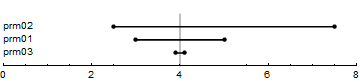
Tornado chart: the global output changes over parameter ranges, sorted by the size of the resulting output range. A vertical line represents the baseline output.
Output-Sensitivity
Suppose the model output is not near zero and that the tornado plot is roughly symmetric around the baseline output measure. Then a better measure of output sensitivity may be the percentage response of the model output to a percentage change in the model input. (Economists call this an elasticity.) Using our previous notation, we may compute this as follows.
Parameter |
Global Output Elasticity |
|---|---|
prm01 |
\(+1.500\) |
prm02 |
\(-0.625\) |
prm03 |
\(+0.025\) |
Local-Sensitivity Analysis
The simplest experiments vary only a single factor at a time. Single-factor experiments can reveal how sensitive a model outcome is to variations in this factor. When the experiment considers on factor values that are near the baseline values, the analysis is consider local.
Global sensitivity can mislead when parameter responses are nonlinear. In this case, the outcomes variations resulting from small changes in paramters may prove more informative. That is, we may conduct local sensitivity experiments in order to show how small changes in a factor change a focal outcome (relative to the baseline parameterization).
Suppose a focal output \(q\) is influenced by a parameter \(p\). Ceteris paribus, we may propose that \(q=m(p)\). This is an abstract representation of the relationship that holds between the focal output and the parameter in our computational model. Call this a univariate metamodel.
Here the metamodel is just a function that maps the parameter to the output. Most of our computational models include substantial stochasticity. In this case, \(m(p)\) will typically describe the average model output (as measured e.g. by the mean or median). Thus we may need to run many replicates at each parameter value in order to produce a good sensitivity measure.
The baseline output \(q_b\) was determined as \(q_{b} = m(p_{b})\), where \(p_b\) is the baseline value of the parameter. If the baseline value is not near \(0\), local variation in the paramter might be and \(1\) percent or \(5\) percent change in the parameter, \(\Delta p > 0\). The experiment for local sensitivity analysis reproduces the focal output measure with a new parameter value, \(p + \Delta p\). The simplest implied sensitivity measure is a slope:
where \(\Delta p\) is a small change in the parameter value. Since \(\Delta p > 0\), this is called a forward difference. When we suspect that this slope may be decreasing (or possibly increasing) in \(p\), it is more common to consider \(p_b - \Delta p\) as well and compute a central difference.
A central difference may be conceptualized as the average of a forward difference and a backward difference. Other related measures are common, including the maximum of the forward difference a the backward difference.
When the output value is not near \(0\), economists often prefer to remove the dependence on measurement units by converting this sensitivity index to an elasticity (by multiplying it by \(p_b/q_b\)).
Univariate Local Sensitivity Table
When we are interested in the output response to multiple parameters, we can compute a sensitivity index for each parameter and report it in a table. This correpondingly multiplies the number of complete simulations we need to run.
Ah Input; More Input!
A univariate local sensitivity measure may offer a poor sense of the consequences of large parameter changes. A univariate-bounds analysis may obscure important response nonlinearities. A possible compromise is to estimate the response based on more values of the parameter. For example, choose mesh points to subdivide \((p_L,p_H)\), and produce output for every mesh point. Unfortunately, if we have multiple parameters to examine, increasing the number of mesh points quickly becomes computationally expensive. One goal of experimental-design techniques is to limit this computational expense while still capturing important information about the model. We will return to this goal.
All Together Now!
An even more computationally demanding analysis considers not just variations in multiple parameters but additionally considers all possible combinations of those parameter values. This can provide important information about how whether simultaneous changes is disparate parameters have important joint effects, but the number of scenarios we must consider rises quite rapidly. For example, even if we want to consider just two different values for each of ten different parameters, this implies \(1024=2^{10}\) different combinations. One way we might reduce the computational burden is to randomly sample these possible combinations. The becomes even more attractive if the sampling prodedure can draw on information about the joint distribution of of these parameters, so that we can more heavily sample the more likely combinations. We will return to this. Looking at how our uncertainty about all the parameters translates into uncertainty about the outputs is sometimes called uncertainty analysis.
Basic Components of Results Reporting
Single factor tables or charts
single-factor sensitivity-analysis table
robustness checks: show that the results are not sensitive to plausible changes in the model
Single-Factor Outcome Tables
For each value of a treatment factor, make a table showing the following:
the treatment value,
the random seed,
and the values of your focus variables at the final iteration (i.e., the values when the simulation stops)
For each value of the treatment parameter, report descriptive statistics for your focus variables. (At the very least, report the mean, standard deviation, and histogram.)
Parameter Uncertainty, Output Sensitivity, and Output Uncertainty
The effect of parameter uncertainty on output uncertainty depends on output sensitivity to the uncertain parameters.
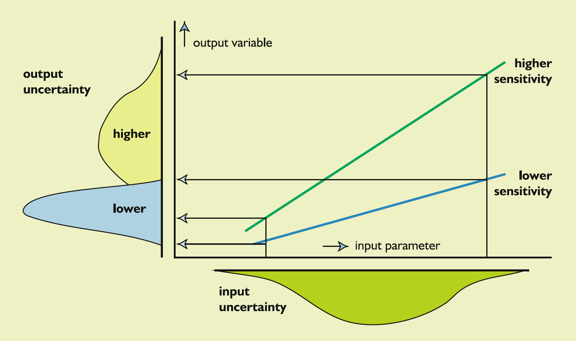
Source: Figure 8.1, [Loucks.VanBeek-2017-Springer]
Design for Multi-Factor Sensitivity Analysis
Design Matrix
- design matrix:
specifies all considered combinations of factor levels that our experiment will consider.
- design point:
a row of the design matrix; a scenario
E.g., if we have just two factors (A and B) with levels A1, A2, B1, B2, B3 a full-factorial design involves six scenarios.
A |
B |
|---|---|
A1 |
B1 |
A1 |
B2 |
A1 |
B3 |
A2 |
B1 |
A2 |
B2 |
A2 |
B3 |
Problem of Dimensionality
Rule: if \(k\) is a big number, then \(2^k\) is a very big number.
Suppose we have \(k\) factors each with just 2 possible levels, that gives us \(2^k\) possible combinations.
- full-factorial (or “fully-crossed”) experiment
considers all \(2^k\) scenarios
- fractional-factorial experiment:
restrict the scenarios considered by imposing constraints (e.g., C=A*B) http://www.itl.nist.gov/div898/handbook/pri/section3/pri334.htm
The same reasoning applies to factors that can take on multiple values. For example, if factor \(i \in [1 .. N]\) can take on \(k_i\) different values, then number of scenarios in full-factorial experiment is
Analysis and Reporting
Response Surface
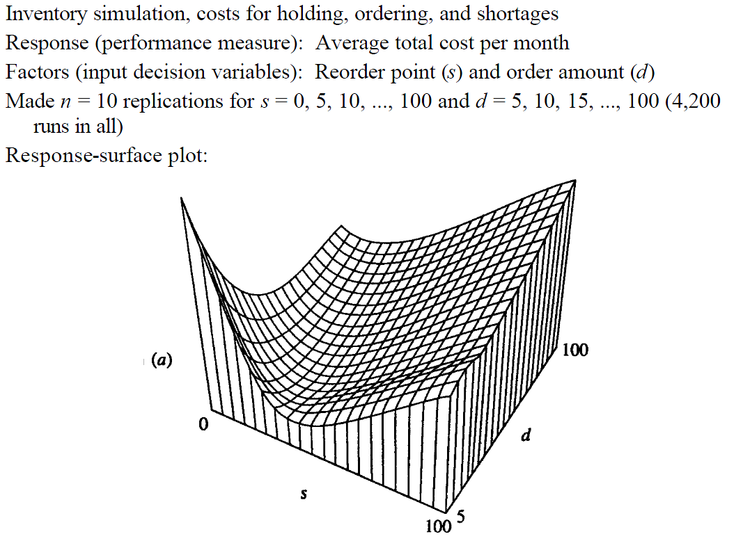
Source: [Kelton-1999-WinSim]
Response Surface: Contours
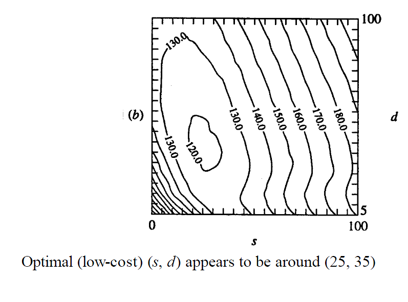
Source: [Kelton-1999-WinSim]
Estimated Response Surface
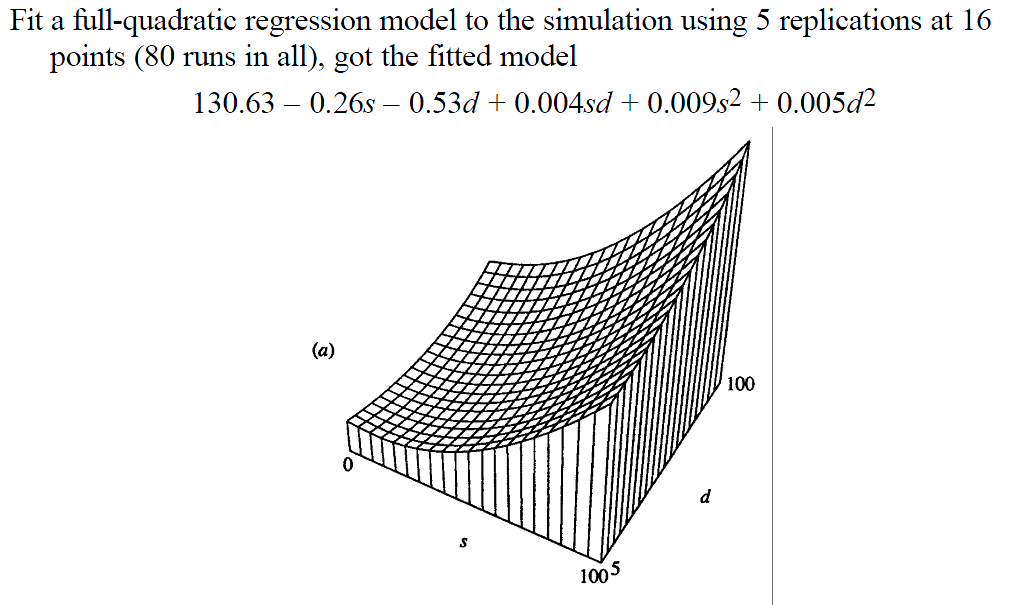
Source: [Kelton-1999-WinSim]
Estimated Response Surface: Contours
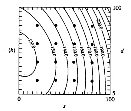
Source: [Kelton-1999-WinSim]
Estimated Response Surface
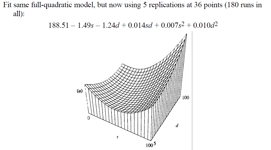
Source: [Kelton-1999-WinSim]
Estimated Response Surface: Contours
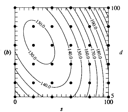
Source: [Kelton-1999-WinSim]
Response of Response
How sensitive is the response to the factors?
- Direct approach (finite differences):
make a run with the factor of interest set to a value
perturb the factor value and make another run
compute slope (difference quotient)
- Indirect approach:
fit a meta-model
consider the partial derivatives
- Single-run methods:
perturbation analysis—move the factor during the run, track new trajectory as well as trajectory if the perturbation had not been made
Graphics
histogram
a standard graphic for simulation outcomes.
puts observations into bins based on their values
plots the number (or relative frequency) of values in each bin.
Histogram
You might construct a frequency histogram for N observations as follows.
Bin your observations into bins B1 ... BN
For each possible bin, Bi, let #Bi denote the number of observations falling in that bin.
Produce the bin relative frequencies bi = #Bi/N
plot the points (i, bi) This is your relative frequency histogram.
Histogram Example
Suppose N = 1000 and you have two bins, for outcomes above (bin 1) or below (bin 2) some segregation measure cutoff.
Suppose 300 observation fall into bin 1.
Then your frequency histogram plots two points: (1,.30) and (2,.70).
Histogram
A histogram can indicate a failure of the data to have a central tendency. (Pareto Distribution)
This is important for our interpretation of our descriptive statistics. E.g., sample mean and sample standard deviation are most useful observations cluster around the mean value.
Meta-Model
response = f(factors)
E.g., summarize with a regression.
Comment: we may have many different responses in a simulation, with a different meta-model for each.
Optimum Response
- Indirect:
fit a meta-model
optimize it using calculus
- Staged
fit a meta-model of low dimensionality
optimize it using calculus
optimum determines a search region for further simulations
- Black box
simulation is a black box function
optimization run by any external tool (e.g., NetLogo's Mathematica link)
Optimization using External Services
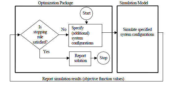
Source: [Kelton-1999-WinSim]
Application: Schelling Segregation Model
Report: Schelling Segregation Model
The simulation model is specified by our code but should be given a supporting description.
Model parameters include:
the size of the world (default: 8 by 8),
the number of agent types (default: 2)
the number of agents of each type (or, the total number of agents and their ratio)
the “happiness cutoff” parameter
the relative size of the different agent classes;
the initial location of the agents.
Treatment Factor and Hypothesis
We can pick any parameter as a treatment factor.
- Illustrative hypothesis:
increases in the happiness cutoff parameter increase the likelihood of a segregated final outcome.
- Turning the hypothesis into a prediction:
given 25 agents each of two agent types and an initial random distribution of agents in the world, a rise in the happiness cutoff increases the final (T=1000) segregation measure.
Randomness and Replicates
Note that this experimental design is probabilistic.
Therefore, for each treatment scenario, you must run multiple replicates.
Typically, each replicate will be based on a different programmer-specified setting of a random seed for the pseudo-random number generator (PRNG) used in the simulation.
Seeding the PRNG
Specification of the PRNG and seed renders the results deterministic (i.e., capable of exact replication).
Therefore, you must record as data the random seed used for each run (along with the values of your treatment-factors) and all user-specified or default settings for maintained parameter values and simulation control options.
Recording the Data
For each run, record the degree of segregation displayed by the resulting agent location pattern.
Report “descriptive statistics” that summarize these experimental segregation findings.
Based on these descriptive statistics, draw conclusions regarding whether or not your hypothesis appears to be supported by your observations.
These descriptive statistics would typically include (at a minimum) the sample mean value, the sample standard deviation, and possibly also a histogram, for the degree of segregation observed across runs.
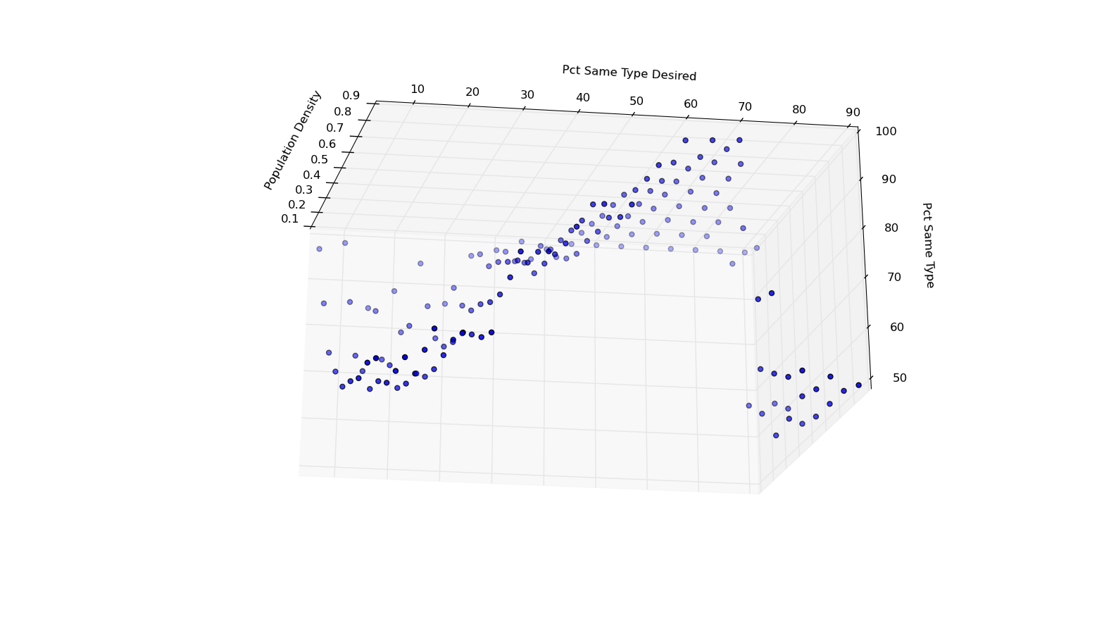
Schelling Model: Response Surface
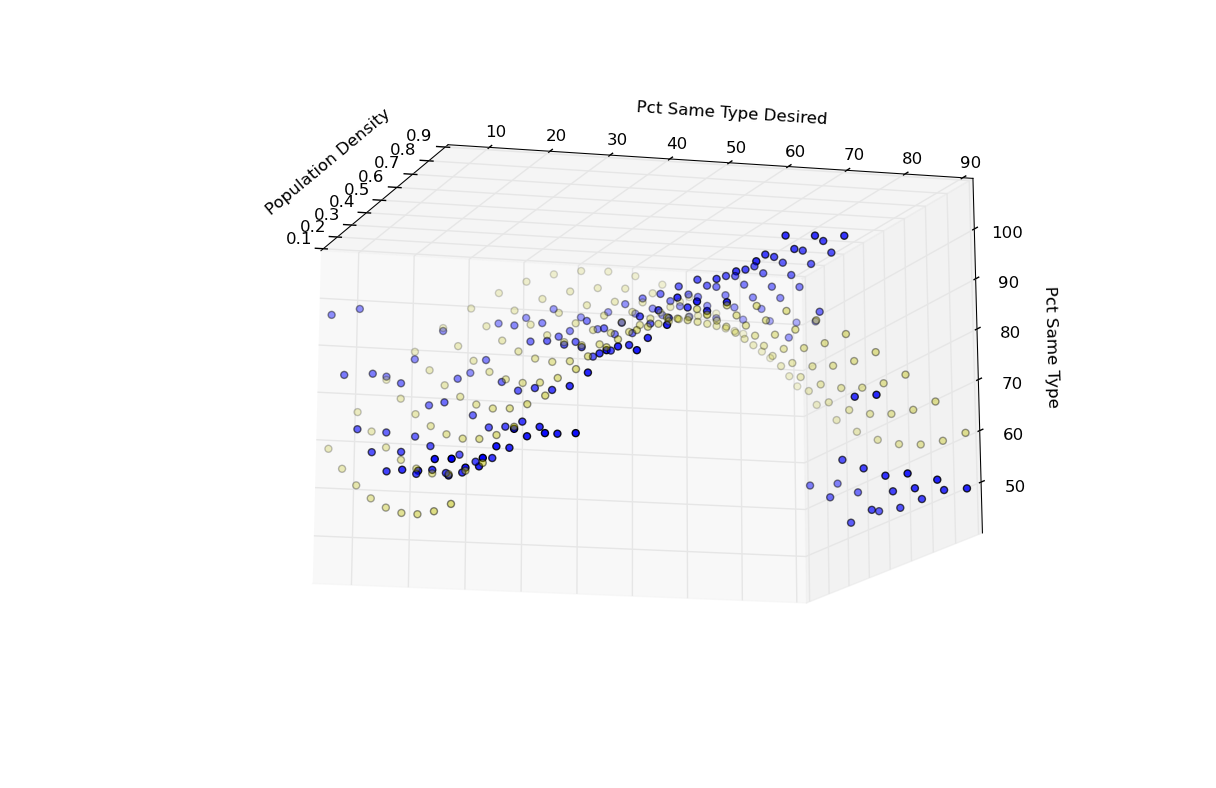
Schelling Model: Response Estimate
After looking at the response surface, seek a meta-model:
- y
pct_same_type
- x1
population_density
- x2
pct_same_type_desired
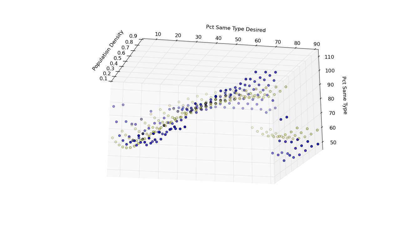
Schelling Model: Responses (blue) v. Fitted Values (yellow)
Schelling Model: Response Estimate
import scikits.statsmodels as sm
y = pct_same_type
x1 = population_density
x2 = pct_same_type_desired
dummy = x2 >= 80
X = np.column_stack((x1, x2, x1**2, x2**2, dummy))
X = sm.add_constant(X)
results = sm.OLS(pct_same_type, X).fit()
print results.summary()
yf = results.fittedvalues
Schelling Model: Response Estimate
==========================================
|            coefficient            prob.|
------------------------------------------
| x1            -73.2431        2.138E-08|
| x2              1.1802        1.080E-13|
| x3             40.3979         0.001051|
| x4             -0.0074        3.685E-05|
| x5            -28.4147        1.077E-12|
| const          73.8049        4.204E-45|
==========================================
Schelling Model: Responses (blue) v. Fitted Values (yellow)
References
Garud, Sushant S., Iftekhar A. Karimi, and Markus Kraft. (2017) Design of Computer Experiments: A Review. Computers and Chemical Engineering 106, 71--95. http://www.sciencedirect.com/science/article/pii/S0098135417302090
Kelton, W. David. (1999) "Designing Simulation Experiments". In (Eds.) Proceedings of the 31st Conference on Winter Simulation: Simulation---A Bridge to the Future - Volume 1, Phoenix, Arizona, United States: ACM.
Ligmann-Zielinska, Arika, et al. (2020) One Size Does Not Fit All: A Roadmap of Purpose-Driven Mixed-Method Pathways for Sensitivity Analysis of Agent-Based Models. Journal of Artificial Societies and Social Simulation 23, Article 6. http://jasss.soc.surrey.ac.uk/23/1/6.html
Loucks, Daniel P., and Eelco van Beek. (2017) Water Resource Systems Planning and Management: An Introduction to Methods, Models, and Applications. : Springer. https://www.springer.com/us/book/9783319442327
Copyright © 2016–2023 Alan G. Isaac. All rights reserved.
- version:
2023-07-14