Feedback in Dynamical Systems
I believe that nothing passes away without leaving a trace, and that every step we take, however small, has significance for our present and our future existence.
—Anton Chekhov, My Life
Not only in research, but also in the everyday world of politics and economics, we would all be better off if more people realized that simple non-linear systems do not necessarily possess simple dynamical properties.
The Exponential Growth chapter introduced core concepts and tools in discrete-time modeling and simulation. A central goal of the present chapter is to augment this modeling toolkit with new programming and data-visualization skills. Once again, the focal model is a simple system-dynamics model of population growth. This time, however, the model more realistically includes feedback from the population level (a stock variable) to its rate of growth (a flow variable).
The core project of the present chapter is the complete development of the basic logistic model of population growth. In this model, the population growth rate is no longer exogenous. In line with the literature on environmental carrying capacity, population changes lead to changes in population growth rates. This chapter demonstrates that this apparently small change in the population growth model can produce substantial changes in system behavior. Furthermore, for certain parameter values, the logistic growth model engenders surprisingly complex dynamics.
State-Dependent Growth Rate
After completing this section, you will be able to do the following.
Explain the concept of environmental carrying capacity.
Explain the Verhulst-Pearl model of population growth.
This section introduces the Verhulst-Pearl characterization of population growth. Their logistic growth model implies that the population growth rate is state-dependent: the current population growth rate depends on the current level of the population. More precisely, the current growth rate depends on the relationship between the current population and its sustainable level.
Recall from the Exponential Growth chapter that an evolution rule describes how a dynamical system that is in one state proceeds to its next state. In the exponential-growth population model of the Exponential Growth chapter, the state of the system is the current population, and one year’s population (along with an exogenous growth rate) determines the next year’s population. In terms of the stock and flow concepts of system dynamics, the flow of net population additions changes the stock of people, which is the world population at a point in time. The present chapter extends the previous model by endogenizing the population growth rate. In the new model, the world population (a stock variable) has a feedback effect on the population growth rate (a flow variable).
Conceptually, the growth rate of a population is the difference between the birth rate and the death rate. The conceptual model of the present chapter embeds an implicit model of constraints on population growth. As a population increases, birth rates eventually fall and death rates eventually rise due to environmental constraints. This implies that the growth rate of the population depends on the level of the population. From a modeling perspective, the population growth rate is no longer exogenous. Instead, it is state-dependent.
Constrained Population Growth
The study of state-dependent population growth rates traces to the mid-1800s. Pierre-François Verhulst famously proposed that the constraints on population growth increase as the population increases. [Verhulst-1845-NMAR] (p.8) proposes that the limited availability of good land might explain these changes. With increasing crowding, the birth rate eventually decreases, and the death rate eventually increases.
This observation readily links Verhulst’s work to modern discussions of environmental carrying capacity, which is the maximum population of a species that a particular habitat can sustain. However, Verhulst did not directly consider the concept of carrying capacity, speaking instead of a natural long-run level of the population. The present chapter adopts a different terminology, the sustainable population, which later sections connect to the mathematical concept of a steady state.
Mathematical Formulation of Logistic Growth
The logistic-growth model of the present chapter draws on a characterization by [May-1974-Science]. The annual growth rate of the population depends on the ratio between the current population (\(P_t\)) and the sustainable population (\(P_{ss}\)). In contrast to the exponential population growth model of the Exponential Growth chapter, there is now a maximum possible growth rate (\(\bar{g}\)). Call this the VP growth parameter. The actual annual growth rate is not constant and does not equal the maximum annual growth rate. The actual population growth rate falls as the population rises, as follows.
To simplify notation, define the relative population (\(p_t\)) to be the ratio of the actual population to the sustainable population (\(p_t = P_t /P_{ss}\)). The logistic growth equation may then be more simply expressed, as follows.
The relative population (\(p_t\)) summarizes the state of this dynamical system at any point in time (\(t\)). That is, the relative population is the state variable for this system. In the logistic-growth model, the population growth rate depends the current population: the growth rate is state dependent. Conceptually, as environmental constraints become increasingly relevant, growth slows. If the constraints are exceeded, population growth can even become negative.
When the population is small relative to the sustainable population, then the relative population (\(p_t\)) is close to zero. In the logistic-growth model, this implies that the population growth rate approaches its maximum (\(\bar{g}\)). However, as the population increases, population growth slows. As the population approaches the sustainable population (where \(p=1\)), the population growth rate falls to \(0\).
To expose the simple evolution rule for the logistic-growth model, solve for \(p_{t+1}\) in terms of \(p_t\). The resulting equation is a useful algebraic summary of the logistic-growth discrete-time dynamical system, which is the focus of the present chapter. This equation summarizes the relationship between next period’s relative population (\(p_{t+1}\)) and this period’s relative population (\(p_{t}\)). The value of \(p_{t}\) in the expression on the right-hand side of this equation determines the value of \(p_{t+1}\) on the left-hand side.
Discrete-Time Dynamics of Logistic Growth
Recall from the Exponential Growth chapter that iteration of an evolution rule produces a system trajectory for a discrete-time dynamical system. In this logistic-growth model, the system trajectory is the relative population trajectory. For example, starting with any given initial relative population (\(p_0\)), repeated application of the evolution rule produces the implied future relative populations. (The corresponding predictions of absolute population levels are \(P_t = P_{ss} p_t\).) Here are the first two iterations along with a general representation of the relationship between relative populations in adjacent years.
Logistic-Growth Map
The corresponding evolution function is a discrete-time Verhulst-Pearl growth function. For any given \(\bar{g}\), this is more commonly called a logistic-growth function or logistic-growth map. [1] Consider the following binary real function. For any given \(\bar{g}\), it transforms a real number (the input) into a real number (the output). Mathematically, this function certainly can be defined on all of the real numbers. However, the conceptual model makes it possible to be more specific: the concept of relative population only makes sense of nonnegative real numbers.
Logistic Function Parameters
Recall from the Exponential Growth chapter that \(\bar{g}\) and \(p\)
in this function expression are the function parameters.
They are bound by the function expression.
That is, the function parameters have meaning only within the function expression,
not outside of it.
For example,
the use of a function parameter \(p\)
in some other function expression
would also be bound by that function expression.
The two uses would have absolutely no relationship to each other.
The use of p in one function expression is completely hidden
from and unrelated to any other function expression.
Computational Logistic-Growth Function
With this mathematical function in hand,
it is time to move on to a computational implementation.
The computational function accepts two inputs:
a real number representing the maximum population growth rate,
and a real number representing the current relative population.
The output is a real number,
which represents the next year’s relative population.
The following function sketch describes
a computational function named nextVP
that performs the desired transformation. [2]
Keep in mind that this function works directly with the relative population,
computed as the current population divided by the sustainable population.
- function signature:
nextVP: (Real,Real) -> Real- function expression:
\(p \mapsto p + \bar{g} * p * (1 - p)\)
- parameters:
\(\bar{g}\), the maximum growth rate
\(p\), the relative population
- summary:
Return the updated relative population: \(p + \bar{g} * p * (1 - p)\).
Create a new project, named LogisticGrowth01.
In the project file, implement the nextVP function,
as described in the function sketch.
During development, test nextVP any way you wish.
Upong completion, implement a more formal test,
and check that nextVP passes this test.
Model Parameters under Logistic Growth
Recall that in simulation modeling,
a model parameter is a constant
in the model implementation that can affect the simulation outcomes.
In the PopulationGrowth01 project of the Exponential Growth chapter,
the population projections depend on two parameters:
the constant population growth rate,
and the initial population.
These are the two model parameters in the project.
In the LogisticGrowth01 project of the present chapter,
the initial population is again a model parameter.
The growth rate is no longer constant,
but a comparable role is now played by the maximum growth rate (\(\bar{g}\)) parameter.
In addition, the logistic-growth model adds third parameter,
reflecting a new consideration.
Population growth now takes place in an environment
characterized by a maximum sustainable population (\(P_{ss}\)).
This planetary carrying capacity is a new model parameter.
Initialization
The Exponential Growth chapter demonstrates two approaches to the introduction of model parameters:
hard coding, and global constants.
Both are somewhat fragile but particularly simple ways
to include model parameters in simulation code.
For the LogisticGrowth01 project,
use global constants for the model parameters.
Name the model parameters P0, Pss, and gmax.
Table t:LogisticParameters specifies crudely plausible values
and provides a model specific interpretation.
name |
value |
meaning |
|---|---|---|
|
8.25 |
initial world population (in billions) |
|
11.5 |
sustainable population (in billions) |
|
0.03 |
maximum annual growth rate |
We would like the values of the model parameters to be plausible. Unfortunately, estimates of the planetary carrying capacity vary substantially. Although a human population of \(10\) billion is a common estimate, the present chapter is slightly more optimistic and raises that by 15% to \(11.5\) billion. You can use this number for the sustainable population (\(P_ss\)). Additionally, assume a maximum population growth rate of 3% per year. This is fairly arbitrary, but as shown below, it produces a plausible initial growth rate. As for the initial population, once again you can research a current value or just use the value suggested in Table t:LogisticParameters.
Augment your LogisticGrowth01 project
to declare and initialize all the model parameters.
Follow the practices introduced in the Exponential Growth chapter.
Conduct any simple test to verify that this setup activity succeeds.
(This may be as rudimentary as
printing the parameters and visually verifying their values.)
Population Projections
Recall from the Exponential Growth chapter that following the setup phase, a typical discrete-time simulation includes an iteration phase. The iteration phase repeatedly executes the simulation schedule. At the core of this schedule is the model update, which implements the evolution rule for the simulation. (This is the computational implementation of the evolution rule derived from the conceptual model.) Each iteration of the model schedule updates the model state.
In the current project,
the model state is simply the relative population.
The model update uses the nextVP function
to update the relative population (code:relpop).
Nevertheless, the ultimate goal is generation of
a sequence of population projections.
This constitutes the next component of the LogisticGrowth01 project:
producing the population projections.
As with the exponential projections,
the logistic population projections will naturally depend on the initial population.
However, as shown below,
population growth now follows a logistic trajectory.
As a result, that dependence diminishes over time.
Approach this population simulation by implementing the following trajectory function sketch.
Here, the specification () -> Sequence indicates that the function
has no input parameters but returns a sequence.
This is the trajectory of population projections.
Note that in this sketch, the function is not pure:
this sequence it produces depends on its environment.
Specifically, it depends on the values of the model parameters.
These parameters occur in the proposed trajectory function as free variables;
their values come from outside the function definition.
- function signature:
trajectory: () -> Sequence- summary:
Do any needed setup of the simulation model.
Compute the initial relative population (
relpop=P0/Pss).Repeatedly (\(50\) times) use
nextVPto update the relative population, making use of the parameterized maximum growth rate.Transform each relative population into an absolute population (
relpop * Pss).Return a sequence containing the entire trajectory of population projections.
Implement the trajectory function described above.
Stretch Exercise:
Refactor the trajectory function
so that it becomes a pure function.
Nonlocal Variables
On the one hand, relying on pure functions is often a good practice: they are easy to understand and have completely predictable behavior. On the other hand, it is desirable for function definitions to avoid hard coding values that we may need to change. The present chapter adopts one possible resolution of this tension: function definitions sometimes may usefully refer to nonlocal variables. (Later chapters explore other approaches.)
A function definition depends on a nonlocal variable when there is an outside influence on the values returned by the function. The value of a nonlocal variable exists outside of the function definition. This implies that the function behavior depends on a potentially changeable part of the environment in which it is executed.
A pure function completely characterizes the relationship between its inputs and its outputs, with no outside influences. In contrast, when a function depends on a nonlocal variable, the relationship between a function’s explicit inputs and its output is unknown until the value of the nonlocal variable is specified. Pure functions are easier to completely understand and therefore are safer to use. Nevertheless, at times impure functions prove convenient, especially early in the development of a program. The rest of this section illustrates one possible use of nonlocal variables in the conduct of simulation experiments.
(Advanced) Free Variables
Nonlocal variables in a computational function resemble free variables in a mathematical function. For example, the variable \(\bar{g}\) is free in the following unary mathematical function. It represents a value that is not supplied as a function argument but is still needed in order to specify the function’s numerical value. This free variable has meaning outside the function expression. In contrast, the variable \(p\) is bound in the following mathematical function. It has no meaning outside the function expression.
A mathematician would say that this function definition
includes \(\bar{g}\) as a free variable,
because \(\bar{g}\) is not bound by the function definition.
This book freely uses this mathematical terminology.
A computer scientist is more likely to say that
an implementation of this function is not pure
unless it replaces \(\bar{g}\) with a number.
Otherwise, gmax is nonlocal to the function definition.
The important point is that, based on this unary function definition alone, the value of \(\bar{g}\) is unknown. This implies that the output of the function is unknown, even when we precisely know the input. Roughly speaking, in order for the output of a function to be completely determined by its arguments, the function definition must contain no free variables. In other words, the definition must be completely closed to outside influences.
To be closed in this way, the definition of a numerical function must completely specify the numerical relationship between the inputs and the outputs. For example, the mathematical function \(p \mapsto p + \bar{g} * p * (1 - p)\) is open to outside influences. It contains the free variable \(\bar{g}\). Unlike the function parameter \(p\), \(\bar{g}\) is not bound in this function definition. This is evident because the variable \(\bar{g}\) does not occur to the left of the maps-to arrow; it is not a function parameter. A function definition containing a free variable is called open, because the return value is open to influences from outside of the function definition.
We might reimplement this function to close it in two ways. One way is to hard code the value of \(\bar{g}\). For example, the function \(p \mapsto p + 0.03 * p * (1 - p)\) is closed. It contains no free variables. Instead, the current project suggests requiring two arguments, so that we work with the binary function \(\langle \bar{g},p \rangle \mapsto p + \bar{g} * p * (1 - p)\). This is also closed.
Producing a Population Trajectory
The above sketch of the trajectory function leaves quite a few details unspecified.
In particular, it does not say when to transform relative into actual populations,
and it does not specify a particular approach to accumulating a sequence
of population projections.
The best approach to these details depends on the implementation language
and the preferences of the programmer.
For example, is some languages it makes sense to create a fixed-size array
and then fill it with values,
while in other languages it is simple and appropriate to
start with an empty sequence and append items to it as needed.
Similarly, in some languages it is most natural to utilize
an imperative looping construct,
while in others a more declarative approach is most natural.
As a result, the following details are only broadly descriptive,
and you should make adjustments as needed in your language of choice.
Introduce two local variables:
say relpop for the relative population and traj for the trajectory.
Initialize relpop to the initial relative population,
and initialize traj to a growable sequence containing just the initial population.
Repeatedly use nextVP to update the relative population,
and repeatedly append the new absolute population to the trajectory.
Once the iteration phase is complete,
return the population trajectory.
Working with the Trajectory
At this point, we have developed all the components needed to run the simulation and collect data from it. The setup phase of the simulation parameterizes the computational model and performs any other needed initialization. It may additionally prepare to collect simulation data. The iteration phase generates a population trajectory. It may additionally collect simulation data. It is natural to implement an activity that handles both phases.
Printing the Trajectory
The following activity sketch describes such an activity, and the subsequent exercise elaborates on its use.
- activity:
printTrajectory- summary:
Print a simulated population trajectory, as produced by the
trajectoryfunction.
This printTrajectory activity
just prints the population values to a computer screen.
Two differing approaches to this activity are
to print each value as it is produced
or to print them all at one go.
For the simulations in this book,
the two approaches are generally equally satisfactory.
Implement the printTrajectory activity, described above.
Note: this activity should print populations, not relative populations. (So scale each relative population by \(P_{ss}\).)
Stretch Exercise: Instead of simply printing the sequence object, print the trajectory values one at a time, one per line.
Data Export Overview
With such a small data set, it may be possible to copy printed output and paste it into a spreadsheet. Nevertheless, simply printing the population projections to a computer screen is neither elegant nor convenient. This section therefore explores a different, more useful approach: writing the data to an output file. This requires a rather small change in the wrap-up stage of the simulation: instead of printing population projections to a computer screen, write them to a file.
Data export can be bulk (i.e., all at once) or incremental (i.e., a bit at a time). Begin thinking about data export by focusing on an end-of-simulation bulk export. In this case, the simulation data much be accumulated by the simulation program. In the present case, there is a single value (the population) that is tracked, and the data is accumulated in a sequence data type, such as a list or array. After the last iteration, the collected data includes is ready for export. As a wrap-up activity, the program can then write this data to file.
- activity:
exportTrajectory- summary:
Write the simulation data to a local file. The data are the simulated population projections produced by the
trajectoryfunction. Write the data as plain text, with one population projection per line.
The Output File
Export of the simulation data to a file involves three conceptual steps: setting up an output file, and writing simulation data to this file, and closing out the interaction with the file. These steps differ substantially across languages and toolkits, and they also differ between incremental and end-of-simulation bulk export strategies. Conveniently, simulation toolkits often offer facilities for data export that require very little effort from the user. In contrast, some programming languages demand a substantial understanding of file handling.
Implement the exportTrajectory activity.
Details:
Create an output folder named out to hold the simulation output.
This chapter assumes that that the out folder
is immediately below the folder containing
the LogisticGrowth01 project’s source code.
Augment this project as needed to export the population projections
to a file named LogisticGrowth01.csv
in the out folder.
For simplicity, just hard code the file path.
Population-Projection Plots
Once we can access the population projections,
it becomes natural to plot them.
Plots often make it easy to see patterns in data
that might be challenging to detect in raw numbers.
This constitutes the next activity.
The following plotTrajectory activity summary leaves out many details,
since the core of this activity is simply to produce a plot.
- activity:
plotTrajectory- summary:
Produce a run-sequence plot of the population trajectory produced by your
LogisticGrowth01project.
Here are some possible ways to execute the plotTrajectory activity.
One may use spreadsheet software to import the exported data and then plot it.
One may use other plotting software to plot this data.
Or, one may use builtin plotting facilities of the programming language
or toolkit used for the simulation.
This last approach can use the simulated sequence directly,
rather than importing the data.
Execute the plotTrajectory activity for the LogisticGrowth01 project.
Compare the new population plot to the plot from the PopulationGrowth01 project.
Figure f:CompareExpLog presents a line chart
based on the LogisticGrowth01 project
along with the one from the Exponential Growth chapter.
The difference between
the projection based on exponential growth
and the projection based on logistic growth
is immediately evident.
In the logistic-growth model,
the population growth rate slows over time,
while in exponential-growth model it does not.
Furthermore, over time the population in the logistic-growth model
appears to be constrained by the fixed sustainable population.
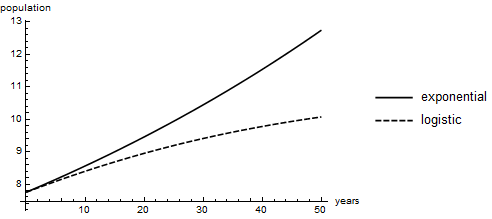
Population Projections (Exponential vs Logistic Growth)
In the exponential-growth model, population continually grows at 1% per year. In the logistic-growth model, population initially grows at about 1% per year, but the growth rate falls as the population approaches its sustainable level.
A Simulation Experiment for the Logistic-Growth Model
The primary goal of this section is to introduce the concept of a simulation experiment. A secondary goal is to use a simulation experiment to elucidate some implications of logistic growth. The project supporting these goals is a very basic experiment with the logistic-growth population model. (Later chapters consider more sophisticated experiments.)
Role of Maximum Growth Rate
The previous section developed a logistic-growth simulation model and produced a set of population projections. These projections eventually diverge substantially from the exponential growth projections of the Exponential Growth chapter. The 50-year forecast from the logistic-growth population model is much lower than the exponential-growth forecast. The new forecast appears more realistic. For example, it better matches the median-variant projection of the United Nations.
The present section considers a natural question about the logistic-growth model: how sensitive are these population projections the model parameterization? This constitutes a research question that may be addressed by means of a simulation experiment. In particular, the maximum population growth rate (\(\bar{g}\)) appears to be a key model parameter for these projections. This section provides a first approach to the question of how changes in the maximum-growth-rate parameter alter the population projections. The approach is experimental: we simulate the population trajectories for various maximum growth rates and then compare them.
Primitive Experimentation
A model parameterization, or scenario, gives a concrete value to each model parameter. During a single simulation run, all of the model parameters retain the same fixed values. In a deterministic system-dynamics model without exogenous inputs, a specifying a model parameterization fully determines the outputs of the simulation.
A simulation experiment compares multiple scenarios. This means that some parameters vary across simulation runs. Simulation experiments allow exploration of a simulation model by exposing how parameter variations affect the system behavior. The parameters selected for variation depend on the particular questions that motivate the experiments. These are the focal parameters of the experiment.
The maximum growth rate is the focal parameter for the present experiment:
we wish to discover how that value of \(\bar{g}\) affects the simulation outcomes.
Unfortunately, in our LogisticGrowth01 project,
this value is hardcoded in the source code.
Nevertheless, as a first approach to experimentation in this model,
briefly try out the following error prone and tedious strategy.
Repeatedly edit the project code to change the
value of \(\bar{g}\),
rerunning the simulation each time.
After each run, recreate the associated run-sequence plot.
The point of this exercise is to gain insight into the limits of this kind of manual approach to simulation experiments. So as you explore this experimentation strategy, you may want to write down some notes about any advantages or disadvantages that you discover.
Copy your entire LogisticGrowth01 project
to a new LogisticGrowth02 project.
Experiment with the new project as follows:
alter the hardcoded maximum annual growth rate
Try the following values: \(1\%\), \(3\%\), and \(6\%\).
Each time you set a new value, rerun the simulation
and illustrate the resulting population projections.
Remember to reset the maximum growth rate to \(3\%\)
when you are done with this exercise.
Some Problems with Primitive Experimentation
Repeatedly changing a hardcoded parameter by hand is a tedious and error-prone approach to experimentation. It requires revisiting the code, finding the hardcoded value, and altering it. This practice becomes increasingly error-prone with more focal parameters. It can be hard to remember the last value set, and there is no hint in the output file of the parameterization used to produce it.
Such primitive experimentation may occasionally prove useful very early in the modeling process. Even so, it is important to move quickly beyond it. This book introduces several better approaches, and the present chapter focuses on a small first improvement: eliminating the repeated changes to a hardcoded value. To accomplish this, this section changes the definition of the trajectory function so that it becomes more pure.
Hard Coded vs Named Parameters
In the Exponential Growth chapter,
the definition of the exponential growth function included
a hard coded 1% population growth rate.
This ensured that nextExponential was a pure function;
the function definition provides all the information
needed to calculate the function’s output for any input.
Functional purity is a very handy:
for any suitable input,
there is never any confusion about what this function should produce as output
(subject to the limits of the computer).
The binary nextVP function of the present chapter is also pure:
given two real inputs, it deterministically produces a real output.
It is closed to all outside influence, and it has no side effects.
However, the LogisticGrowth01 project hard codes the model parameters.
As illustrated by the previous exercise,
for the current simulation experiment, this has drawbacks.
Although the maximum growth rate must remain constant during any simulation run,
the experiment requires it to change across simulation runs.
A hardcoded model parameter becomes an annoyance whenever
a simulation experiment requires repeatedly resetting it to varied values.
It is wise to assume that any attempt
to coordinate such code changes eventually will fail.
To address this,
let us refactor the trajectory producing function,
making it less dependent on its execution environment.
Refactoring the Trajectory Computation
Specifically, use the following function sketch
to implement a trajLG02 function,
which handles the trajectory computation.
This is a ternary function:
it accepts the three model parameters as inputs,
and produces a simulated logistic-growth population trajectory.
(The function summary provides descriptive guidance,
but produce the population trajectory however you wish.)
- function signature:
trajLG02: (Real, Real, Real) -> Sequence- parameters:
\(\bar{g}\), the VP maximum growth rate parameter
\(p_\text{ss}\), the sustainable population
\(p_0\), the initial population
- summary:
Compute the initial relative population, \(r_0 = p_0/p_\text{ss}\).
Partially apply \(\mathrm{nextVP}\) to produce \(f = r \mapsto r + \bar{g} \, r \, (1 - r)\).
Iteratively (\(n\) times) apply \(f\) to produce the relative-population trajectory \(\langle r_0, f[r_0], \dots, f^{\circ 50}[r_0] \rangle\).
Return the corresponding population trajectory. (Each population scales a relative population by the sustainable population: \(r * p_\text{ss}\).)
Implement this trajLG02 function in your LogisticGrowth02 project.
Also test your implementation to ensure that it behaves as expected.
Optional: Include a fourth input parameter: the number of population projections to produce.
When computing a population trajectory,
the trajLG02 function depends on the value assigned to \(\bar{g}\).
Applying this function to a new value of \(\bar{g}\)
produces a different population trajectory.
Each change in \(\bar{g}\) produces a new trajectory.
The trajLG02 function provides an abstract representation of all of these trajectories.
This allows us to easily experiment with changes in the maximum growth rate.
Take advantage of this by executing the following collectTrajectories activity.
- activity:
collectTrajectories- summary:
Produce a useful collection of three logistic-growth population trajectories, one each for the following values of \(\bar{g}\): 1%, 3%, and 6%. Use
trajLG02to produce each trajectory. Keep the sustainable population and initial population at the baseline values, given in Table t:LogisticParameters.
Abstractly, producing the collection of trajectories
is effectively a mapping operation,
using a partially applied trajLG02 function
over a sequence containing the maximum growth rates.
The result of such a mapping operation is a sequence of trajectories.
However, you may store the three trajectories in any way you find
most helpful for the following exportTrajectories activity.
which is to export the trajectories to a CSV file.
- activity:
exportTrajectories- summary:
After executing the
collectTrajectoriesactivity, write the three population trajectories to a columnar CSV file namedLogisticGrowth02.csv. That is, put one trajectory in each of its three columns.
Finally, consider the following plotTrajectories activity.
This activity can also benefit from the collectTrajectories activity.
After producing the collection,
use the lessons learned in the LogisticGrowth01 project
to plot each trajectory.
- activity:
plotTrajectories- summary:
After executing the
collectTrajectoriesactivity, produce a run-sequence plot for each trajectory. If possible, place the plots in a single chart, along with a helpful legend.
Execute the exportTrajectories activity.
Execute the plotTrajectories activity.
Compare the three trajectories.
Experimental Results
Figure f:varyMaxPopGrowth illustrates typical results from completing this exercise. Raising the maximum growth rate produces initially more rapid growth, so the corresponding population projections are higher. Fifty-year population projections are clearly sensitive to the maximum growth rate in the logistic model of population growth.
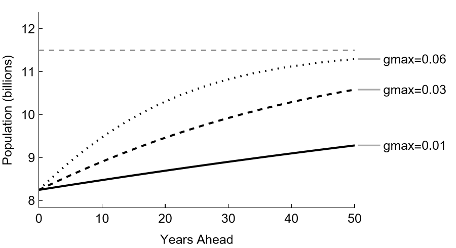
Logistic Population Projections (Various \(\bar{g}\))
(Advanced) Complex Logistic Growth
This section further explores the logistic-growth function by considering radically different values of the Verhulst-Pearl growth-rate parameter. The new values cannot even remotely describe human population growth, which correspondingly is not the focus of the present section. Rather, this section explores a few mathematical concepts along with some more advanced programming skills. Readers may prefer to skip this section for now and return after mastering a few more chapters.
Steady State
The LogisticGrowth02 project demonstrated that,
over the chosen forecast horizon of 50 years,
fairly small changes in the growth rate parameter
have fairly large effects on the population projections.
In this sense sense,
population projections are sensitive to this parameter.
However, longer term projections eventually converge to the sustainable population.
In this sense,
the population projections are eventually similar,
despite these changes in the parameterization.
Although changing the maximum growth rate changes the speed of convergence,
it does not change the sustainable population.
This implies that in the LogisticGrowth02 project,
a long-run population projection does not depend on the maximum growth rate.
This observation leads us toward the concept of a steady state of a dynamical system. A steady state is a state that, in accordance with the evolution rule of the system, does not change over time. If a deterministic dynamical system is in a steady state, it stays there.
In LogisticGrowth02 project,
the sustainable population (\(P_{ss}\))
determined the long-run outcomes of the logistic-growth simulations.
Furthermore, \(P_{ss}\) is a steady-state population.
That is, if the population equals \(P_{ss}\),
it will not change.
Restated in terms of populations relative to the sustainable level,
if the relative population equals \(1.0\), it will not change.
Steady States as Fixed-Points
From a system-dynamics point of view, it is natural to speak of a steady state of a system. The related concept from mathematics is a fixed point of a function. When applying a function to some value reproduces that value, the value is a fixed point of the function. So a steady state is a fixed point of an evolution function.
Recall our logistic-growth function for the relative population: \(p \mapsto p + g \, p \, (1 - p)\). Iterating this function produces a trajectory for the relative population. It is easy to show that this system has a steady state, where the output value of this function is the same as the input value. The steady-state values solve the following equation in \(p\).
This equation expresses the requirement that the function produce a value equal to its input. Given \(g \neq 0\), we can see by substitution that both \(0.0\) and \(1.0\) are steady-state values of this dynamical system. That is, they are fixed points of the logistic-growth function.
Recall that a relative population of \(1\) corresponds to a population that equals the sustainable population. A system that attains the sustainable population stays there. As we might guess intuitively, a population of \(0\) is also a steady state: an extinct species stays extinct.
The LogisticGrowth02 project produces \(50\) years
of population projections for various maximum growth rates.
In each case,
longer projections eventually converge to a relative population of \(1\).
None of these trajectories converge to 0.
This convergence behavior indicates that
these two fixed points have very different dynamical properties.
In the LogisticGrowth02 project,
the value \(1\) is a stable fixed point of the logistic functions:
when the population is near the sustainable population, it approaches it.
Equivalently, the value 1 is an attracting fixed point,
or attractor, in these dynamical systems.
In contrast, the value 0 is an unstable fixed point:
when the population is a bit above \(0\), it continues to grow.
Equivalently, we say that the value 0 is a repelling fixed point,
or an repellor, of these dynamical systems.
A New Experiment
Despite its simplicity, the Verhulst-Pearl logistic growth function can produce more complicated behavior than monotone convergence toward the steady state. As a first observation to support this claim, consider the possibility of overshooting the steady state when \(g > 1\). For example, confirm that \(\mathrm{nextVP}[1.5,0.8]=1.04\), exceeding the steady-state value of \(1.0\). A subsequent iteration then produces a value below the steady state. It seems that at large values of \(g\), a logistic-growth function can produce a trajectory that fluctuates around a steady state. This is the case, as demonstrated by the following exercise.
Create a new LogisticGrowth03 project,
copying code from LogisticGrowth02 as needed.
Produce three logistic growth trajectories,
this time for \(g\) values of
\(1.9\), \(2.0\), and \(2.1\).
(This time, do not transform the results into a population series.)
For our present purposes,
it suffices to work with half as many iterations as before.
Plot each trajectory. Summarize any changes in behavior that you discover.
To support this exercise,
and more generally to allow varying the number of iterations,
slightly refactor the trajectory function to take the following three arguments:
the maximum growth rate, an initial value, and a number of iterations.
Call this new function iterVP.
- function signature:
iterVP: (Real, Real, Integer) -> Sequence- parameters:
\(g\), the VP growth parameter
\(p_0\), the initial population
\(n\), the number of iterations
- summary:
Let \(f = p \mapsto p + g \, p \, (1 - p)\).
Iteratively (\(n\) times) apply \(f\) to produce the trajectory \(\langle p_0, f[p_0], \dots, f^{\circ n}[p_0] \rangle\).
Return the entire trajectory.
Experimental Results
Figure f:varyMaxPopGrowth2 illustrates typical results from completing this exercise. The now larger values of the maximum growth rate produce quite different behavior than before. Letting \(g = 1.9\) still produces a convergent trajectory, but it fluctuates around the steady state. Raising \(g\) to \(2.0\) still produces a convergent trajectory, and it still fluctuates around the steady state, but it converges more slowly. (Much more slowly, as it turns out.) Raising \(g\) still further to \(2.1\) produces a new behavior. The trajectory still fluctuates around the steady state, but it does not appear to converge.
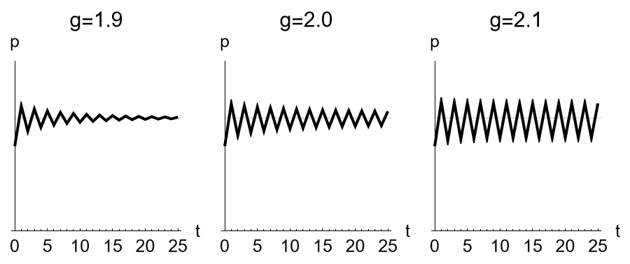
Logistic Population Projections (\(p_0=0.75\); various \(g\))
Picturing Fixed Points
Why does that last case (\(g = 2.1\)) appear not to converge? Let us explore this with a common visualization of the fixed points of this logistic function. Create an ordinary function plot in the Cartesian plane, along with a \(45^\circ\) line. At its fixed points, a function plot crosses the \(45^\circ\) line. In this case, the function is the evolution function of a dynamic system, so these points of intersection identify the possible steady states. Figure f:logistic-vp210 provides an illustration.
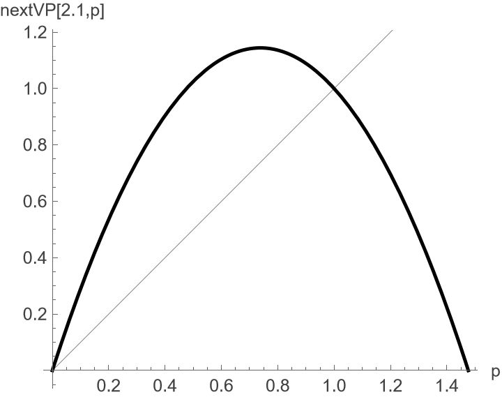
Logistic Function (\(g = 2.10\))
As expected from the algebraic discussion of the fixed
points of the nextVP function,
we always see the two lines intersect at \((0,0)\)
and \((1,1)\).
This remains true even at much higher values of gmax;
the locations of the fixed points do not depend on gmax.
However, this does not mean that the behavior of the model is unchanged.
Now each fixed point is unstable,
because the function slope is too steep.
It is natural to be a bit puzzled that the steady state is no longer an attractor. This results from the steeper slope of the logistic-growth function. For a fixed point to be an attractor, the slope of the function at that point must be less than one in absolute value. Increases in \(gmax\) increase the slope of the logistic-growth function at its fixed points. The sustainable population is still a steady state for the system, but it is no longer a stable steady state. To be a stable fixed point, the slope must lie in \((-1\,..\,1)\), but now the slope is \(3.25\) at \(p=0.0\) and \(-1.25\) at \(p=1.0\). Raising the maximum growth rate makes the function steeper and steeper at the two steady states, until eventually the steady state at \(1.0\) is no longer stable.
(Optional) Reproduce Figure f:logistic-vp210, using a plot domain of \([0.0\,..\,1.45]\).
Periodic Attractors as Fixed Points
So the steeper slope explains the new lack of convergence, but what explains the apparently periodic behavior? To approach this question, suppose this function actually does have periodic values, recurring every two periods. Begin a function iteration with one of these points, apply the logistic-growth function to it, and then apply the logistic-growth function to the result. This reproduces the original point. That is, such a periodic point is a fixed point of the twice iterated function.
As a convenient notation, for any unary function \(f\), represent the twice iterated function as \(f^{\circ 2}\). Now let \(f = p \mapsto \mathrm{nextVP}[2.25, p]\), so that \(f^{\circ 2}\) is a twice iterated logistic function. We may then use the same graphical approach as before to reveal the fixed points of this iterated function. Simply plot \(f^{\circ 2}\), and search for its intersections with the \(45^\circ\) line.
Of course any fixed point of \(f\) must also be a fixed point of \(f^{\circ 2}\). So the new plot must rediscover the original steady-state points. And as shown in Figure :name: f:logistic-vp2x225, the iterated function \(f^{\circ 2}\) indeed has fixed points at \(0\) and \(1\). But in addition, there are now \(2\) more intersections: the two periodic points (near \(0.71\) and \(1.17\)).
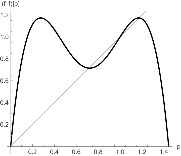
Function Plot for Twice-Iterated Logistic Growth (\(g=2.25\))
This is an example of a periodic attractor, and the two additional fixed points are called periodic points. More specifically, the two points can alternate in a period-2 cycle. What is more, this two cycle is attractive. We see that visually because the slope of \(f^{\circ 2}\) at the periodic points is clearly less than unity. So if we start at some other value of \(p\), the trajectory will approach the period-2 cycle over time. This is an example of a limit cycle: the cycle is the limiting behavior of the trajectory.
Longer Cycles
Our discovery of period-2 cycles shows that our iteration of our simple logistic-growth function can generate surprisingly complicated dynamics. It is natural to wonder if longer cycles are possible. For example, does \(f^{\circ 4}\) have any additional fixed points? Letting \(g = 2.25\), a quick plot reveals no additional fixed point. Nevertheless, there is more to come.
In your LogisticGrowth03 project,
produce one additional logistic growth trajectory,
this time for \(g = 2.5\).
As before, in order to match the illustration below,
let the initial value for your function iteration be \(0.75\).
Another Experimental Result
Figure f:logistic-gmax250 illustrates typical results from completing this exercise. Letting \(g = 2.5\) produces a fluctuating trajectory around the nonzero fixed point, but this time there appears to be a 4-cycle.
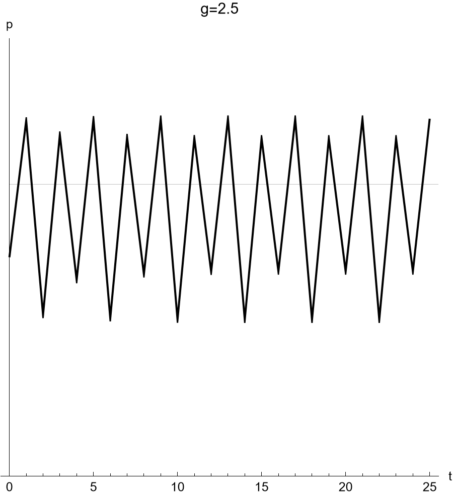
Logistic Population Projections (\(g = 2.50\))
Letting \(f=p\mapsto nextVP[2.5,p]\), one may try to shed light on this with a function plot. The plots of \(f\) and \(f^{\circ 2}\) are easy to interpret: the 1-cycles and 2-cycles are clearly unstable (due to the steep slopes there). Making a useful plot of \(f^{\circ 4}\) is challenging: While it is possible to make out the four points of the 4-cycle, this is not easy unless the plot is very big (or zooms in). It is time for a better approach.
Period Doubling
We found that when the VP growth parameter is \(2.10\),
the trajectory is attracted to a period-2 limit cycle.
Two points have long-run relevance for this system,
which alternates between them.
When we increase the VP growth parameter to \(2.5\),
the trajectory is attracted to a period-4 limit cycle.
Four points have long-run relevance for this system.
In the face of this discovery,
it is natural to ask whether such period-doubling continues to result
from increases in the VP growth parameter.
The answer is yes—and with faster and faster period doubling.
(This is called a period-doubling cascade.)
When we raise gmax to \(2.55\),
the trajectory is attracted to a period-8 limit cycle,
but unfortunately this is almost impossible to discern with such plots.
It becomes harder and harder to detect these oscillations visually.
Brute Force Computation of Limit-Cycle Points
In addition to such basic problem of visual discrimination, regularities in the limiting behavior of a function iteration may be concealed by the early behavior. To deal with this problem, simulation analysis often incorporates a burn-in period. This involves discarding initial iterations of a dynamic system in order to better focus on the behavior it ultimately settles into. The burn-in period is the number of discarded iterations.
There is another problem:
computers generally work with approximate numbers.
If computers were capable of infinitely precise computations,
the actual trajectory would approach its limit cycle over time.
Unless the initial point is a periodic point, however,
the process of convergence would continue forever.
However, given the limitations of digital computers,
an actual cycle between approximate numbers emerges after a finite number of iterations.
This suggests a strategy for numerically finding periodic points:
run the simulation for a while,
and then search for repeating values towards the end of the trajectory.
That is, discard the first part (“prefix”) of a long trajectory,
and then examine the final segment for periodic behavior.
One approach to producing such a post-burn-in sequence segment
is illustrated by the following segmentVP function sketch.
- function signature:
segmentVP: (Real, Real, Integer, Integer) -> Sequence- parameters:
\(g\), the VP growth parameter
\(p_0\), initial value for trajectory
\(n_1\), the length of the trajectory prefix to discard
\(n_2\), the length of the trajectory segment to keep
- summary:
Let \(f = p \mapsto p + g \, p \, (1 - p)\).
Starting with \(p_0\), iteratively (\(n_1\) times) apply \(f\) to produce the value \(p_{n_1} = f^{\circ n_1}[p_0]\).
Return
iterVP[g,p_{n_1},n_2 - 1].
This is a good start, but if this detects a limit cycle,
much of the sequence segment is likely to be redundant.
The limit-cycle points are the set (i.e., no repetitions) of the elements in the sequence segment.
In principle, discarding the duplicates is fairly trivial,
since most language include some facility for easily doing this.
In practice, however, we again run into the limitations of floating-point computations:
multiple nearly equal approximate numbers may represent a single limit-cycle point.
For this reason,
let us treat numbers that are very similar as actually being the same.
One way to do this is to discard the final decimal places of each computer number
prior to comparing them.
The following sketch of a nudupes function captures this idea.
- function signature:
nodupes: RealSequence -> RealSequence- parameters:
\(\mathrm{xs}\), the input sequence of real numbers
- summary:
Let \(\mathrm{ys}\) be the values of the \(\mathrm{xs}\), but rounded to 12 decimal places.
Return the unique elements of the \(\mathrm{ys}\).
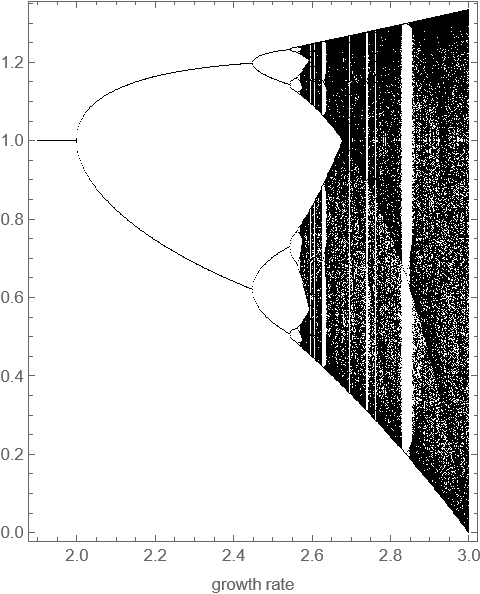
A bifurcation is the doubling of the period of the limit cycle.
A bifurcation plot
is popular way to illustrate the effects of changing the parameter gmax.
For each value of g,
it plots the limit-cycle points determined as above (but often with longer trajectories).
It displays the points that are occur in the limit cycle.
This will be only 1 point for \(g < 2\),
but will then move into a period-doubling cascade,
including more and more points until a visual display of all the points becomes impossible.
Once we choose the values of the VP growth parameter to consider, we are ready to create a bifurcation plot. This is a scatter plot showing the periodic (limit-cycle) points for each value of the VP growth parameter. This chapter describe a brute-force approach to producing this plot, while acknowledging that this has a number of problems. For example, how do we know if we have chosen an adequate burn-in period? And, how do we know if we have chosen an adequate segment length? Nevertheless, brute-force approaches to the creation of a bifurcation diagram remain far the most common. Experimentation indicates that the following brute-force approach should quickly produce a revealing plot for this logistic-growth model. Figure f:periodicPointsLogistic illustrates a typical result of this brute-force approach.
Bifurcation Plot:
Implement the segmentVP and nodupes functions
described above.
Consider at least 500 evenly spaced values of the
VP growth parameter (\(g\)) in the closed interval \([1.9\,..\,3.0]\).
For each value, use nodupes and segmentVP
to produce the implied limit-cycle points.
(Try a segement length of 250 after droping a prefix of 1750.)
For each g, plot the \(\langle g, p \rangle\) pairs,
for each associated limit-cycle point (\(p\)).
Use the horizontal axis for the VP growth parameter values
and the verical access for the associated limit-cycle point values.
Periodic Points (Iterated Logistic Growth)
On to Chaos
Examining the bifurcation diagram, we can easily detect the first three period doublings discussed above. But then the situation quickly becomes much messier. In fact, above about \(2.57\), many situations arise where there is no periodicity at all. This is the realm of chaotic dynamics. The behavior of this simple nonlinear dynamical system is no longer just complicated, it is complex.
This complex behavior has spawned a very large literature. Of particular interest is that, when dynamics are chaotic, this simple, deterministic, nonlinear system becomes effectively unpredictable. To pin this down a bit, it means that even miniscule changes in the initial conditions can lead to utterly divergent long-run behavior. To put it more provocatively, long-run prediction effectively becomes infeasible.
Summary and Conclusions
Conclusion
This book repeatedly considers four steps: developing a conceptual model, implementing it as a computational model, using the computational model to run a simulation, and examining the data produced by the simulation. This chapter illustrated these components of simulation modeling by developing a simple model of logistic population growth.
Logistic Growth vs Exponential Growth
As a population-growth model,
the logistic-growth model incorporates the concept of a sustainable population.
This chapter linked the concept of a sustainable population
to the concept of environmental carrying capacity,
which is the population that the available habitat can sustain indefinitely.
Recognizing the limits to population growth add realism
and leads to very different population projections than the exponential-growth model.
For example, the simulation experiment of the LogisticGrowth02 project
found that very different initial rates of population growth
produce divergent short-run population projections,
yet the long run forecast does not depend on the growth-rate parameter.
Exploration, Resources, and References
Supplementary Exploration
Use a spreadsheet to produce a 50-year population projection, under the same population assumptions as above. In the Spreadsheet Introduction supplement, find details for this spreadsheet exercise in the discussion of step-by-step population projection. Compare your spreadsheet results to the simulation results above.
Change the
trajectoryfunction in theLogisticGrowth01project so that is it a pure function, which consumes three arguments. (You may keep the hard coded trajectory length.) Make the implied changes elsewhere in the project code. (Each use oftrajectorynow needs three arguments.)Each step, in addition to writing the current population to
LogisticGrowth01.csv, write the current relative population. Write the two numbers on a single row, separated by a comma. (This data is in CSV format.)Reproduce Figure f:compareExpLog, which compares the outcomes under exponential growth and logistic growth.
Reproduce Figure f:varyMaxPopGrowth, which compares the logistic-model outcomes under three different values of
gmax. Predict what will happen if you extend the simulation another \(50\) years: will the final predictions be even further apart, or will they be closer together? Explain the reasoning behind your hypothesis. Run simulations to test your hypothesis.Impose the constraint that the input to the
nextVPfunction is nonnegative. (The best approach to this depends on the programming language.)Create a slider for the initial population (\(p_0\)). Use this slider for simple model exploration. Does the initial population matter for the long-run behavior of the system?
Instead of hard coding the output file name in the exporting activity, introduce it as a global constant (say,
outputFile).(Advanced) In the
LogisticGrowth02project, instead of hard coding the number of iterations in thetrajLG02function, make it another function parameter (say,nIter). How does this affect how you produce your plots?(Advanced) In the Spreadsheet Introduction supplement, do the regression exercise on estimating the sustainable population for the U.S.
Additional Resources
Population Models and History
The American Museum of natural history describes the history of human populations in a video entitled Human Population Through Time. The United Nations maintains a World Population Prospects website, which includes data visualizations of world population trends. The website also provides access to population data and research in population studies.
For an introductory discussion of the concept of carrying capacity, see the Wikipedia entry. [Sayre-2008-AAAG] discusses varied uses of the term carrying capacity, and [Hui-2006-EcolMod] clarifies the distinction between population equilibrium and carrying capacity. [Arrow.etal-1995-EcoEcon] and [Niccolucci.etal-2007-EcolEcon] relate carrying capacity and environmental sustainability. [Wilson-2003-Knopf] offers a readable discussion of the sustainability of human populations. [Wilson-2003-Knopf] estimates that Earth’s arable land can sustainably support 10 billion vegetarians. Many estimates are much lower. Some estimates are much higher. Sustainability estimates are strongly influenced by assumed standards of living and forecasts of technological change.
The population models in this book use a system dynamics approach rather than an agent-based approach. [Geard_etal-2013-JASSS] offer an agent-based analysis, with an emphasis on demographic structure. Their model is implemented in Python, and they provide access to their code.
The Logistic Map
Wikipedia includes helpful introductions to the Logistic Map and to step plots. [Feldman-2012-OxfordUP] provides a more detailed yet extremely accessible introduction to both topics, and his chapter 7 discusses population models and a logistic function. [May-1974-Science] and [May-1976-Nature] provide early discussions of chaotic dynamics in very simple nonlinear systems. On YouTube you can find (as of 2025) a nice, leisurely introduction to bifurcation theory by Nils Berglund. [Jafari.etal-2021-IJBC] discusses practicable approaches to improving bifurcation diagrams.
Chapter 3 of [Kingsland-1995-UChicago] provides a detailed history of the introduction of the logistic hypothesis into research on population growth. [Rosling.Rosling.Rosling-2018-Flatiron] provide a data-rich discussion of the importance of such considerations to human population forecasts. The United Nations Department of Economic and Social Affairs provides world population data and projections, along with helpful charts displaying some of this data. [Cramer-2002-WP] explores the historical development of logistic regression, with connections to the early work of [Verhulst-1838-CMP].
Cobweb Charts (Step Plots)
A popular alternative visualization of these periodic outcomes is provided by a cobweb chart, which includes a type of step plot. Given a sequence \((x_0,x_1,x_2,\ldots,x_n)\), a cobweb chart plots stepped line segments between the points \((x_0,x_1)\), \((x_1,x_1)\), \((x_1,x_2)\), and so on. Conventionally, cobweb chart plots additionally start and end on the \(45^\circ\) line by adding the point \((x_0,x_0)\) at the start and \((x_n,x_n)\) at the end.
Draw two segments each iteration.
Given the value \(p_0\) we can produce the value \(p_1=f[p]\),
which allows us to draw segments
from \((p_0,p_0)\) to \((p_0,p_1)\)
and then from \((p_0,p_1)\) to \((p_1,p_1)\).
In order to do this however,
we need access to both values.
In the code, use two global variables
(named p and plag) to store these values.
Change the project code to include p and now plag as global variables.
Each iteration, update both of these globals
before you update your plot.
To support this exercise, introduce a new global variable named lagrelpop,
which holds the lagged value of relpop.
The step activity should now set lagrelpop to relpop
before updating relpop.
Overlay a step plot on your function plot,
producing a cobweb chart.
(You may add plotting an initial point to the plot setup.)
After each step,
the plot update should plot the new point of the function graph
and then a new point of the \(45^\circ\) line.
Once the step-plot code is functional,
re-examine our last experiment.
Do 5 iterations at a time and watch
how the plot changes.
After about \(20\) function iterations,
there are now more visible changes in the step plot.
To pursue this observation a bit further, without clearing the global variables, clear the plots and then plot a few more iterations. In the time-series plot, this renders the period-2 cycle readily visible as an oscillation between two values. In the step plot, we see an unchanging square, reflecting this oscillation between the two period-2 points.
Global Variables
Recall that simulation models in this book typically include a setup phase that sets the model parameters and initializes any global variables. The initial values of the global variables often depend on the model parameters.
At this point,
there are two global variables in the computational model.
The first is relpop,
which holds the current population relative to the sustainable population.
(So relpop is the source-code variable that corresponds
to the \(p\) in the mathematical discussion above.)
Given the values of model parameters,
initialize relpop to P0 / Pss.
Second, as a convenience,
the model includes a global variable named ticks.
This variable should track the number of iterations of the model step,
so initialize ticks to \(0\) during the setup phase.
In addition to setting the values of the model parameters,
the setup phase includes the initialization of any global variables.
For example,
the exponential growth model of the Exponential Growth chapter
introduced the current population as a global variable of the model.
This offers a simple way to track the state of the population during a simulation.
In the present chapter,
a similar role is played by the relative population (relpop).
This is the ratio of the population to the sustainable population.
Whenever it might be needed,
the actual population may be recovered as Pss * relpop.
name |
initial value |
meaning |
|---|---|---|
|
|
relative population |
Incremental Data Export
An alternative to end-of-simulation bulk export is incremental export of the data. This is particularly advantageous when a simulation generates very large amounts of data. For incremental export, the setup phase includes preparing an output file and writing the initial data. The iteration phase then appends data to this output file after each simulation step.
For incremental export,
the setup phase typically includes a little file preparation.
For example,
the setup phase typically discards any existing data
from prior runs of the simulation.
In addition, for incremental data export,
the setup phase typically writes
the initial model state to the output file.
The following summary of a setupFile activity
captures these considerations.
- activity:
setupFile- summary:
Set up an empty output file.
Write the initial population as plain text to the first line of the empty output file.
For incremental export,
the end of the iteration phase should write new data to the output file.
Even though the data-export step is currently very simple,
this section introduces a recordStep activity to handle it.
For the current model,
execution of the recordStep activity
appends a number to the output file by writing it on its own line.
That number is the current population.
- activity:
recordStep- summary:
Open the output file for appending.
Append the current population to the file, on its own line.
Close the output file.
This file handling exercise is optional. You may use BehaviorSpace to export your data.
Create a setupFile activity, as described above.
Create a recordStep activity, as described above.
For simplicity, simply hard code the file path
(e.g., "out/LogisticGrowth01.csv").
Naming the Output File
The earlier discussions of file handling assumed that the name of the output file is hardcoded. This is fine when a deterministic simulation runs under a single parameterization. Multiple simulation runs create some new considerations when it comes to data export, since each simulation run will overwrite the last output.
For example, suppose each simulation writes a population trajectory to file. It would be possible after each simulation run to copy the output file to a new location, but this is again tedious and error prone. Two possible responses are either to alter the code to run the entire experiment and write all the resulting projections to a single file or to ensure that each parameterization produces a unique output file. For the moment, consider the latter.
When a parameter changes across simulation runs,
it should be possible to somehow link the parameterization to the output file.
This book explores a number of approaches to this problem,
but here is the simplest:
specify the parameterization in the name of the output file.
This eliminates one source of potential confusion in the analysis of the
results of the initial simulation experiment.
Any change in the value of the gmax parameter
should automatically change the name of the output file.
In the LogisticGrowth03 project,
create an outfile variable
that holds the path to the output file.
In the setup phase (e.g., in the setupFile activity),
set the value of outfile to LogisticGrowth-gmax_{gmaxpct}.csv,
where {gmaxpct} represents gmax as a percentage.
(Multiply gmax by 100.)
For example, when gmax is 0.03,
the filename should be LogisticGrowth-gmax_3.csv.
Modify the data export code to use this new filename.
Revised Plot Code
Revised Slider
A goal of this section is to consider a
more extensive set of values for gmax.
Create a new LogisticGrowth03 model
by copying the LogisticGrowth02 model.
Do not make any further changes to the old model.
Alter the slider in the new model
to extend from 1% to 300%.
Visualizing Logistic Population Growth
GUI Experimentation
Create a slider widget for interactive experimentation.
Create a button widget for simulation control.
Create an animated time-series plot.
This section emphasizes interactive visual exploration of the logistic-growth model. It therefore focuses on the development of a useful graphical user interface (GUI). After completing this section, you will be able to create GUI buttons for simulation control. You will also be able to use sliders for interactive experimentation. The focal output of this section is a time-series plot, which provides a helpful visualization of the simulation data. A core goal is increased familiarity with the basic GUI facilities of your chosen language or simulation toolkit.
Widgets for Simulation Control
So far, this project has utilized a command line interface in order to run the population simulations. This is quite flexible, but for interactive experimentation it is not fully satisfactory. For one thing, it may involve tedious and error prone typing at the command line. Additionally, it complicates sharing of the model: command-line usage may appear obscure to new users of the model. A standard remedy for these problems is to add a GUI interface to the model.
Clickable buttons are a particularly common GUI widget.
(A GUI widget is a graphically presented control or display element,
such as a control button, a slider, a text box, or a plot element.)
Models built with simulation toolkits often provide
buttons that allow even a new user to easily set up and run the simulation.
Correspondingly,
add a button for simulation control
to the LogisticGrowth02 project.
Add a GUI button labeled Run Sim
to your LogisticGrowth02 project.
For the moment, this Run Sim button should just
execute the printTrajectory activity.
Once you have created your button,
use it to run your simulation.
This should print the same propulation projections as before.
Sliders
Watch this video on slider creation.
One popular approach to interactive parameter manipulation, particularly in the early phases of simulation modeling, is the addition of control widgets. A slider is a control widget that provides a simple graphical interface for setting a variable’s value. It is a natural choice when we wish to experiment with a parameter that can take on a range of numerical values. A slider typically specifies a default value for a variable and then allows a user to reset that value within a constrained range.
The next goal of this section is to demonstrate the use of a GUI slider for interactive model experimentation. Accordingly, the next exercise adds to the model GUI a slider that controls the maximum growth rate. Remember that model parameters should not change during the iteration phase of the simulation. So, use this slider only to influence the model setup, which must take place after the slider is set.
Add a GUI slider to your LogisticGrowth02 project.
This should control the value of the maximum growth rate
with the new global variable (gmax).
Design the slider so that it can take on at least
the values of 1%, 3% (the default), and 6%.
(A later section considers additional values.)
Time-Series Plot
The Exponential Growth chapter illustrated the use of dynamic plots for the display of simulation results. This section continues that practice and then discusses widgets for GUI experimentation with a simulation model.
Prepare for this by adding a time-series plot of the population projections
to your LogisticGrowth02 model.
Creation of the time-series plot should closely follow
the discussion in the Exponential Growth chapter.
Plotting must incorporate one substantive difference from that previous work:
since the core simulation produces a trajectory for the relative population,
you must transform the data to plot the population levels.
Rely on the previous discussion of the printTrajectory activity
to guide this transformation.
First, review the discussion of plotting in the the Exponential Growth chapter.
Then, add a time-series plot to the LogisticGrowth02 project.
This plot should display the annual population projections
produced by the population simulation.
(If possible, this should be a dynamic plot.)
The title of this plot should be "Time Series".
To populate the plot, implement a runsimG activity
that modifies your runsim activity by adding plotting.
Remember to include plotting of the initial model state in the setup phase.
Use this runsimG activity
to plot the annual population projections for \(50\) years.
Refinements
In anticipation of future models,
add a few refinements to the existing LogisticGrowth02 code.
Isolate the plot setup,
and bundle the new simulation schedule.
Implement an activity that sets up the plot;
call it setupPlotTS.
This activity should plot the initial population
and, if possible, set the axes limits and labels.
As a minor convenience,
package the entire simulation schedule (including plotting)
into a new go activity.
(This will execute your step activity.)
Refactor your runsimG activity
to repeatedly execute this new go activity.
GUI Exploration of the Logistic Growth Model
During the early stages of simulation modeling,
interactive experimentation is common.
The GUI of the LogisticGrowth02 project
is now rich enough to support this.
Set the new slider for gmax to the default values of \(0.03\),
and use the Run Sim button to run the simulation.
Next, use the slider for gmax
to double the maximum growth rate to \(0.06\).
The behavior of the population is very similar,
but convergence to the \(P_{ss}\) is faster.
Also use the slider for gmax to cut the maximum growth rate to \(0.01\).
The behavior of the population is again very similar,
but convergence to the \(P_{ss}\) is slower.
The results should not be surprising:
they resemble Figure f:CompareExpLog.
This rapid process of interactive experimentation
illustrates the usefulness of plots, buttons, and sliders
for model exploration.
Invariance of the Fixed Points to the Growth Rate
It may be a difficult to distinguish the \(45^\circ\) line
from the function plot when gmax is \(0.03\).
As you increase the value of gmax,
the gap between the two plots becomes more visible.
Now, consider a substantially higher value of gmax,
which makes it much easier to detect the two fixed points.
Use the slider to set gmax to 1.6.
Figure f:vpfp160 provides an illustration of the two fixed points
of the logistic-growth function when gmax is \(1.6\).

Fixed Points of nextVP (\(g=1.6\))
New Short-Run Behavior at Higher Growth Rates
name |
default value |
range |
increment |
|---|---|---|---|
|
\(0.03\) |
\([0\;..\;3]\) |
0.01 |
As a small convenience for the upcoming experiments,
make two changes to the model GUI.
In addition to setting up the simulation,
the Set Up button should now set up both charts.
Furthermore, add a Go 5 button to the model,
which runs go a total of \(5\) times.
Setup the model and run the simulation for \(5\) iterations.
Figure f:vpts160 shows that the time series
produced at such a high value of gmax:
is qualitatively different:
the simulation no longer produces a monotone sequence.
However, increases in the number of iterations show that
the population still converges to \(Pss\).
The sustainable population is still a stable steady state
(attractive fixed point).

Time Series from nextVP Iteration (\(\bar{g}=1.6\))
References
Arrow, Kenneth, et al. (1995) Economic Growth, Carrying Capacity, and the Environment. Ecological Economics 15, 91--95. http://www.sciencedirect.com/science/article/pii/0921800995000593
Cramer, J.S. (2002) "The Origins of Logistic Regression". Tinbergen Institute Working Paper 2002-119/4. https://papers.tinbergen.nl/02119.pdf,http://dx.doi.org/10.2139/ssrn.360300
Feldman, David P. (2012) Chaos and Fractals: An Elementary Introduction. : Oxford University Press.
Geard, Nicholas, et al. (2013) Synthetic Population Dynamics: A Model of Household Demography. Journal of Artificial Societies and Social Simulation 16, 8. http://jasss.soc.surrey.ac.uk/16/1/8.html
Hui, Cang. (2006) Carrying Capacity, Population Equilibrium, and Environment's Maximal Load. Ecological Modelling 192, 317--320. http://www.sciencedirect.com/science/article/pii/S0304380005003339
Jafari, Ali, et al. (2021) A Simple Guide for Plotting a Proper Bifurcation Diagram. International Journal of Bifurcation and Chaos 31, 2150011-1--2150011-11. https://doi.org/10.1142/S0218127421500115
Kingsland, S.E. (1995) Modeling Nature. : University of Chicago Press. https://press.uchicago.edu/ucp/books/book/chicago/M/bo3630803.html
May, Robert M. (1974) Biological Populations with Nonoverlapping Generations: Stable Points, Stable Cycles, and Chaos. Science 186, 645--647. https://science.sciencemag.org/content/186/4164/645
May, Robert M. (1976) Simple Mathematical Models with Very Complicated Dynamics. Nature 261, 459--67.
Niccolucci, Valentina, Federico M. Pulselli, and Enzo Tiezzi. (2007) Strengthening the Threshold Hypothesis: Economic and Biophysical Limits to Growth. Ecological Economics 60, 667--672. http://www.sciencedirect.com/science/article/pii/S0921800906005416
Rosling, Hans, Anna Rosling Roennlund, and Ola Rosling. (2018) Factfulness: Ten Reasons We're Wrong About the World---and Why Things Are Better Than You Think. : Flatiron Books.
Sayre, Nathan F. (2008) The Genesis, History, and Limits of Carrying Capacity. Annals of the Association of American Geographers 98, 120-134. https://doi.org/10.1080/00045600701734356
Verhulst, P. (1838) Notice sur la Loi que la Population Poursuit dans son Accroissement. Correspondance Mathematique et Physique 10, 113--121.
Verhulst, Pierre-Fran,cois. (1845) Recherches Mathematiques sur la Loi d'Accroissement de la Population. Nouveaux Memoires de l'Academie Royale des Sciences et Belles-Lettres de Bruxelles 18, 1--41. http://gdz.sub.uni-goettingen.de/dms/load/img/?PPN=PPN129323640_0018&DMDID=dmdlog7
Wilson, Edward O. (2003) The Future of Life. : Knopf Doubleday Publishing Group.
Appendix: Logistic Growth (Details and Hints)
Implementing the Logistic Growth Projects in NetLogo
This section provides guidance for an implementation of the projects in the Logistic Growth chapter, using the NetLogo programming language.
LogisticGrowth01 (NetLogo)
Based on your reading in the Introduction to NetLogo supplement,
create a new model file named LogisticGrowth01.nlogo.
The Code tab of this file should hold all the code for the LogisticGrowth01 project.
Implementing nextVP (NetLogo)
Add a nextVP function (i.e., reporter procedure) to the project,
relying on the function sketch provided in the Logistic Growth chapter.
Then test that the implementation is correct.
The function sketch specifies that this function transforms two real values into another real value. Recall that your NetLogo code can largely ignore information about numerical data types: NetLogo includes only a single numerical data type, which is used to represent both real numbers and integers. Recall from the NetLogo Programming supplement that a NetLogo function definition includes a space-separated list of function parameters, enclosed in brackets. There is one function parameter for each argument the function will need.
After adding an implementation of nextVP to the project file
(LogisticGrowth01.nlogo), test it.
At the very least,
confirm that your nextVP implementation passes the following test,
which you can add to this project’s Code tab.
to test-nextVP
  type "Begin test of `nextVP` ... "
  if (0 != nextVP 0.03 0) [error "bad next relpop fr 0"]
  if (0 != nextVP 0.01 0) [error "bad next relpop fr 0"]
  if (1 != nextVP 0.03 1) [error "bad next relpop fr 1"]
  if (1 != nextVP 0.00 1) [error "bad next relpop fr 1"]
  print "`nextVP` passed."
end
Once it passes your tests and you are satisfied with your implementation,
compare it to the following NetLogo code.
This is one possible NetLogo implementation of nextVP.
Parameterization
Introduce the model parameters as global variables.
Recall from the PopulationGrowth01 project
that NetLogo requires that you first declare
these variables (with globals) and only
subsequently set their values.
So add the declaration globals[P0 Pss gmax]
near the top of the Code tab.
This declares three global variables.
Initialization is typically handled during
the setup phase of the simulation model.
For this project,
create a separate setupGlobals procedure
to set the values of the model parameters.
In the conceptual model,
each parameter is a real number.
However, you can ignore this detail,
since NetLogo has only a single numerical data type.
Check your work at the NetLogo command line
by running your setupGlobals procedure
and then printing the values of the parameters.
Recall that NetLogo does not offer a facility to ensure parameter constancy. Nevertheless, model parameters should not change as the simulation runs. it is entirely up to the you to ensure that these values remain unchanged after initialization.
Trajectory for LogisticGrowth01
Start your definition of the trajectory function
by calling setupGlobals.
That ensures that properly initialized parameter values are available to the function,
which depends on them.
(It is not a pure function.)
After that, there are many possible ways to implement a good trajectory function.
You may take any approach,
but start by following the description in the Logistic Growth chapter.
In NetLogo,
the list data type provides the most common way
to incrementally collect a data series.
(See the NetLogo Programming supplement for a detailed discussion.)
So use a list to hold the population trajectory.
Recall that the Introduction to NetLogo supplement covers iterative list building.
Keep in mind from the prerequisite reading about NetLogo lists that
the list command is often required to create a list,
since the alternative syntax using brackets can only be used with literal values
(not with variables or computations).
For example, although [20] creates a list because 20 is a number literal,
[10 * 2] does not work.
Instead, use (list (10 * 2)) in this case.
Similarly, use (list pop0) when initializing the trajectory with the initial population.
After that, repeatedly use lput top append updated values during the iteration phase.
(Remember that lput produces a new list with an appended value,
so it should generally be used with set.)
A correctly implemented trajectory function will pass the following test.
With the trajectory function in hand,
it is trivial to execute the printTrajectory activity.
As the crudest approach to this activity,
enter the following at the NetLogo command line: print trajectory.
As a slightly more interesting command-line approach, follow the general
list-iteration example
in the NetLogo Programming supplement to print one item per line in the Command Center as follows:
foreach trajectory print.
This code simply applies the general approach to iterative printing,
using a particular list of values.
Writing the trajectory to file is very similar to printing it,
but file management will require two extra steps:
preparing the file for data export,
and closing the file once we are finished.
The approach considered here requires the following NetLogo commands:
carefully, file-delete,
file-open, file-print, and file-close.
Review these in the NetLogo Dictionary,
and recall that the NetLogo Programming supplement covers them in detail.
NetLogo cannot directly overwrite an existing file.
The equivalent action in NetLogo is to delete the existing file
and then write a new file with the same name.
This process creates a slight conundrum,
since trying to delete a non-existent file is an error.
An idiomatic solution, as illustrated in the NetLogo Programming supplement,
is to use NetLogo’s carefully command
to wrap the file-delete command as follows:
carefully [file-delete "out/LogisticGrowth01.csv"] [].
(For this project, you may just hard code the filename.)
This deletes the file if it already exists,
but the use of carefully ensures that
it does not produce an error if the file does not exist.
Recall that NetLogo’s print command
can simply print a numerical value,
without requiring prior conversion to a string.
Additionally, it prints linewise,
appending a carriage return (to terminate the line).
The same is true of file-print.
This means that, aside from the new file management code,
the core of the exportTrajectory activity is
a very small adaptation of the printTrajectory activity:
just replace print with file-print.
Implement an exportLG procedure to support
this activity.
This procedure should have an input parameter for the trajectory it will export.
After adding this procedure to the Code tab,
execute the exportTrajectory activity by entering the
following code at the NetLogo command line:
exportLG trajectory.
Next, produce a run-sequence plot of the trajectory.
The Logistic Growth chapter suggests several approaches to this activity.
Drawing on the experience gained during the previous project (PopulationGrowth01),
add a plot to the new model’s Interface tab,
Recall that a preliminary for any plotting activity
is adding (by hand) a plot widget to the Interface tab of the project file.
So right-click in the main window of the Interface tab,
and create this plot widget.
As a good practice whenever plotting, provide labels for the axes.
In addition, add a plot name (say, Logistic Growth) during the widget creation process.
This will appear at the top of the plot widget.
With the plot widget in place,
it is time to add the plotting code to the Code tab.
As in the previous project,
divide the plotting activity into two components:
setting up the chart, and plotting the points.
Create two command procedures for these components:
say, setupPlotLG and plotLG.
Begin by copying the setupPlot procedure from the PopulationGrowth01 project.
Next, add set-current-plot "Logistic Growth" as the first line
of the procedure body.
This simply identifies the plot widget,
using the name you gave it during the widget creation process.
(In later models, with multiple plot widgets, this practice becomes important.)
Also add a new second line: clear-plot.
This ensures that plotting begins with a blank canvas,
even if you have previously plotted on it.
Define the plotLG procedure with one input parameter:
the list to be plotted.
The first line of the procedure body should call setupPlotLG.
Then, plot each population projection.
You should now be able to execute the plotTrajectory activity
by entering the following code at the NetLogo command line:
plotLG trajectory. (Try it.)
This runs the simulation and plots the resulting population trajectory.
However, since GUI building is so easy in NetLogo,
let us add one refinement to this model.
Using what you learned from the Introduction to NetLogo supplement about adding widgets in the Interface tab,
add a single button by right-clicking in the main window
and picking the Button option.
This opens a widget-creation dialog.
Enter Run Simulation as the display name and
plotLG trajectory as the commands.
Pressing OK then creates a button that,
when pressed, runs the population simulation and plots it.
LogisticGrowth02 (NetLogo)
Begin the LogisticGrowth02 project by
copying the LogisticGrowth01 project.
Refactor the trajectory computation,
as described in The Logistic Growth chapter.
Implement the new computation as a trajLG02 function.
Remember to test your work.
A properly implemented trajLG02 function,
which takes three arguments,
must pass the following test.
to test-trajLG02
  type "Begin test of `trajLG02` ... "
  let _traj (trajLG02 gmax pss pop0)
  if (pop0 != first _traj) [error "bad trajectory"]
  if (51 != length _traj) [error "bad trajectory"]
  set _traj (trajLG02 0.0 pss pop0)
  if (pop0 != last _traj) [error "bad trajectory"]
  print "`trajLG02` passed."
end
Once your trajLG02 passes this test
and you are satisfied with your implementation,
compare it to the following NetLogo code.
This is one possible NetLogo implementation of trajLG02.
With trajLG02 in hand,
it is possible to approach the collectTrajectories activity.
There are many possible approaches to this activity.
In every case,
we must produce the three needed trajectories,
one for each value of \(\bar{g}\).
Abstractly, this effectively maps a partially applied trajLG02 function
over a sequence containing the maximum growth rates.
The result of this operation is a sequence of trajectories.
Concretely, even though map is a builtin function,
a new NetLogo programmer may be more likely to build up a list of trajectories
inside a for statement.
This is a fine approach,
but let us use map.
This is usually the most idiomatic way to map a function across a list of values.
The following gmaxExperiment function takes this approach,
but it then goes further.
Instead of simply returning the list of trajectories,
it uses them to produce a table mapping experiment names to trajectories.
The gmaxExperiment function takes one argument,
a sequence of maximum growth rates.
It produces a trajectory for each one of these,
using NetLogo’s builtin map function
and this project’s trajLG02 function.
Note how NetLogo’s arrow notation makes it very
easy to create the function needed by map.
The resulting unary anonymous function is a partially applied version of trajLG02,
where the maximum growth rate is the only needed input.
Using table:from-list,
it is possible to produce a table directly from
a list of key-value pairs.
The trajectories will be the values.
In order to have useful keys,
we produce a list of descriptive names,
one for each experiment.
Another use of map then allows us
to pair each name with its trajectory,
giving us the needed list of key-value pairs.
We report the table produced from this list of key-value pairs.
To complete the exportTrajectories activity,
we turn to the to-file command in NetLogo’s csv extension.
He we support the activity with an exportTrajectories procedure,
which accepts the table produced by gmaxExperiment as input.
For now, to keep things simple, the output file is hard coded.
(How might you produce a more informative filename?)
To get the list of trajectory names,
apply the table:keys function.
To get the list of trajectories,
apply the table:values function.
To use csv:to-file to produce a columnar CSV file,
we first need to transpose the list of trajectories.
Here we use the unzip function from the fp extension,
as discussed in the NetLogo Programming supplement.
Prepend the list of names to the new list of rows,
so that there will be column headers in the CSV file.
Then write the result to your file.
Finally, proceed to the plotTrajectories activity.
As usual, add a plot widget to the Interface tab.
However, this time in the widget dialog,
delete the default plot pen and check the legend checkbox.
Support this activity with the following plotLG02 procedure,
which consumes the table of input trajectories produced by gmaxExperiment.
(Plot setup remains unchanged.)
Since there are multiple trajectories,
we will use multiple plot pens—one for each trajectory.
In is convenient to use the trajectory name for the pen name.
Use NetLogo’s set-plot-pen-color command to set each pen to a random color,
picked as one-of basecolors.
Finally, plot each trajectory just as in the LogisticGrowth01 project.
It is now possible to execute the plotTrajectories activity
by entering the following code at the NetLogo command line.
As a refinement, add a button to the Interface tab
that runs this code.
plotLG02 gmaxExperiment [0.01 0.03 0.06]LogisticGrowth02 with BehaviorSpace
Generally speaking, when it comes to experimental results, relying on the programmer to produce output files by detailed file management is not the NetLogo way. Instead, users are typically expected to rely on BehaviorSpace to generate output for simulation experiments. To do this in an idiomatic way requires changing the model a little to allow BehaviorSpace to record each output as it is produced.
In order to support a BehaviorSpace experiment,
introduce relpop as a global variable,
and add its initialization to setupGlobals.
In addition, add a procedure that simply uses nextVP to update relpop.
In NetLogo models, this is conventionally called go.
Add this code in the Code tab of your model. Then open BehaviorSpace as described in the Introduction to NetLogo supplement, and press the New button. Give the experiment an informative name, and then fill in the experiment dialog as follows. (Hover a mouse over the bold dialog text for more guidance, if needed.)
Vary variables:
["gmax" 0.01 0.03 0.06].Measure runs:
relpop * Pss.Setup commands:
setupGlobals.Go commands:
go.Time limit:
50.
Do not forget to include a time limit for this model! Press the OK button to close the dialog and create the experiment. Press the Run button, add a file name for "Spreadsheet" output, and press the OK button. This runs the experiment and produces a CSV file, which you may use for additional analysis or visualization.
This discussion illustrates some trade-offs in the use of BehaviorSpace. On the plus side, there is less and simpler code. On the minus side, the programmer loses control over the formatting of the exported data. In addition, we had to introduce an otherwise unneeded global variable. Finally, for the BehaviorSpace experiment, it is less obvious how to produce all three trajectories in the Interface tab.
LogisticGrowth03 (NetLogo)
The LogisticGrowth03 project needs access to
the trajectories produced by iteration of of the Verhulst-Pearl logistic-growth function.
Provide these by implementing the iterVP function
described in the Logistic Growth chapter.
(This task reuses skills developed in implementing trajLG02.)
Here is one approach.
After partially applying nextVP to the VP growth parameter,
the following implementation uses fp:iterate to do the function iteration.
Exporting the data and using other software to plot it
is always an option.
However, the following discussion focuses on plotting in the Interface tab.
In the same way as in previous projects,
add a plot widget to this project’s Interface tab.
It may be named Trajectory. (Do not delete the default plot pen.)
Since the new trajectories are more volatile than in the LogisticGrowth02 project,
plotting multiple trajectories together in a single plot frame becomes too messy.
Therefore, plot one trajectory at a time.
In order to support the plotting activity,
write a plotTrajLG03 procedure that consumes
the VP growth parameter (g)
and produces a run sequence plot in the Trajectory plot widget.
For now, plot the trajectory produced by iterVP[g, 0.75, 25].
Include whatever setup you find useful.
Here is one approach.
For ease of experimentation,
as described in the Introduction to NetLogo supplement,
add a slider for the VP growth parameter.
Name it gmax,
and allow \(300\) values from \(0.01\) to 3.00.
Since the gmax parameter is now an interface global variable,
ensure that it is not additionally declared in globals.
(Recall the discussion of interface globals in the Introduction to NetLogo supplement.)
Now you should be able to use the slider to set gmax
and then run plotTrajLG03 gmax from the command line
to produce the corresponding run-sequence plot.
For even greater ease of experimentation,
add a Run Simulation button to the Interface tab.
Let this button execute plotTrajLG03 gmax.
Using the new slider and button,
conduct the three-trajectory experiment of the LogisticGrowth03 project.
That is, one at a time,
set the gmax slider to \(1.9\), \(2.0\), and \(2.1\)
and the display the resulting trajectory.
After noting the differences between these plots, try one more:
set the slider to \(2.5\), and once again plot the resulting trajectory.
The next goal is to create a bifurcation plot.
To begin this project,
first determine the possible limit-cycle points for
any given value of the VP growth parameter.
As suggested in the Logistic Growth chapter,
approach this by creating a segmentVP function
and a nodupes function.
Follow the chapter’s function sketches.
Here is one approach.
In this example code, segmentVP relies on the fp extension,
which as always must be declared at the top of the Code tab
(using the extensions keyword).
The first step is to partially apply the nextVP function
to the VP growth parameter in order to produce a unary real function.
To cheaply drop the trajectory prefix,
this example uses fp:iterate-last.
(This produces only that final value of the iteration.)
To produce the needed segment, however, we then need to collect subsequent terms.
The fp:iterate function accomplishes this
exactly as in the previous iterVP implementation.
NetLogo’s remove-duplicates reporter makes it simple to produce a list of unique values.
However, we wish to discard misleading noisy differences between numbers that
result only from the finite precision of floating-point computations.
Given a list of floating-point numbers, this nodupes function
uses NetLogo’s precision function to round them to the \(12\)-th decimal place.
Two values that are equal at this level of precision are treated as actually equal,
so nodupes retains only one value for the two of them.
As described in the Logistic Growth chapter,
the segmentVP and nodupes functions
nicely support the creation of a bifurcation plot.
For the production of this plot,
add a second plot widget to the Interface tab of your LogisticGrowth03 project.
Set the name to Bifurcation Plot,
and edit the mode of the default pen to be Point.
(This is the pen mode needed for a scatter plot.
You may alternatively set this during any plot setup with the command
set-plot-pen-mode 2.)
You can put the actual plot setup code and plotting code
either directly in the plot widget or in a new plotBifurcations procedure.
The discussion here focuses on the content of such a procedure.
Since there are now two plot widgets,
setup should use NetLogo’s set-current-plot command to activate
the desired widget.
It is also a good idea to execute the clear-plot command,
so as to start from scratch.
Lastly, this plotting procedure should produce and plot all the desired points.
Since we have no other use for these points,
there is no need to collect them all (e.g., in a list).
Instead, it simply plot each point as it is produced.
For each considered value of the VP growth parameter (g),
produce the periodic points as nodupes (segmentVP g 0.75 1750 250).
Using this g as the first coordinate and the periodic points as second coordinates,
plot a small point for each pair (using NetLogo’s plotxy command).
Repeat this for enough values of g to ensure an informative bifurcation plot.
The following plotBifurcations implementation produces a bifurcation plot
very similar to that in the Logistic Growth chapter.
Extending the Logistic Growth Model (NetLogo)
You may use BehaviorSpace to export the data. (See the Introduction to NetLogo supplement for an introduction to BehaviorSpace.)
Additional Resources
NetLogo’s documentation is very good, but sometimes additional resources can help new users. Recall that the Introduction to NetLogo supplement includes a short introduction to BehaviorSpace. A web search turns up good video discussions of BehaviorSpace. Here are a couple to start with.
The following video discusses NetLogo’s csv extension.
Implementing the Logistic Growth Projects in Python
This section provides guidance for an implementation of the projects in the Logistic Growth chapter, using the Python programming language.
LogisticGrowth01 (Python)
Create a new model file named logistic_growth01.py.
This file should hold all the code for the LogisticGrowth01 project.
Implementing nextVP (Python Specifics)
Add a nextVP function to the project,
relying on the function sketch provided in the chapter text.
Then test that the implementation is correct.
The function sketch specifies that this function transforms
two real values into another real value.
In Python, type annotations are always optional,
but for the present project,
let us add type annotations to indicate the intended use of this function.
Python programmers typically use the float data type
to represent mathematical real numbers.
So use float to annotate the function parameters and return type.
Recall that a Python function definition
includes a comma-separated sequence of function parameters,
enclosed in parentheses.
There is one function parameter for each argument the function will need.
Adding type annotations does not change this structure.
However, instead of the simple signature nextVP(gmax, x),
the function signature now becomes nextVP(gmax: float, x: float) -> float.
The new function signature feels more visually noisy,
but it is more informative about the intended use of this function.
Only you can determine whether this trade-off is worthwhile is a specific setting.
However, note that there is an additional advantage to providing type hints in this way:
there are a variety of static type checkers for Python that can analyze
the consistency of the type hints that you provide.
(A particularly popular Python type checker mypy.)
After adding an implementation of nextVP to your LogisticGrowth01 project file,
test it.
At the very least,
confirm that your nextVP implementation passes the following test,
which you can add to the project file.
def test_nextVP():
    assert (POP0 == nextVP(0, POP0))
    assert (0 == nextVP(GMAX, 0))
    assert (1 == nextVP(GMAX, 1))
Once it passes your tests and you are satisfied with your implementation,
compare it to the following Python code.
This is one possible Python implementation of nextVP.
Parameterization
For the LogisticGrowth01 project,
introduce the model parameters as global variables.
Recall from the PopulationGrowth01 project
that in Python an assignment statement
can both declare and initialize a variable.
So declare and initialize three global variables
near the top of the project file.
Check your work at the Python command line
by importing the three parameters
and then printing their values.
Model parameters should not change as the simulation runs. However, recall that Python does not offer a facility to ensure this constancy. It is therefore entirely up to the programmer to ensure that these values remain unchanged after initialization. Nevertheless, the inability to better enforce constancy can be troubling. When this becomes a real concern, Python can offer related functionality.
For example, type hints can assist in communicating your intent,
and type checkers can examine the consistency of your type hints.
Since Python 3.8, variables may be annotated as Final.
Although this annotation is not enforced at runtime,
it is used by static type checkers such as mypy.
(See PEP 591 for details.)
Therefore, as you introduce the three parameters,
consider adding the following type hint: Final[float].
As before, this indicates that the values assume Python’s float numerical data type,
but now the use of Final states in addition that the values should never change.
Note that in order to use Final as a type hint,
you must first import it from Python’s typing module.
Keep in mind that such type hints do not affect how the program runs.
Nevertheless, a static type checker (such as mypy) can check them for consistency.
Simulating Logistic Population Growth
The next task is to use the model parameter and the
nextVP function to produce population projections.
Start your definition of the trajectory function
by using the model parameters to compute the initial relative population.
This is the setup phase.
After that, there are many possible ways to implement the iteration phase.
You may take any approach,
but start by following the chapter description.
Use a list to hold the population trajectory.
Recall from the prerequisite reading about
Python lists
that you may simply use brackets to create a list.
For example, [] creates an empty list.
As another example, [20] or [10 * 2]
or x=10; [x * 2] all create the same list,
which contains a single number.
For the current projection,
approach iterative list building by means of the repeated of
of the append of lists.
Remember that append changes an existing list by appending a value.
Be sure to test your implementation of the trajectory function.
As usual, writing tests is a critical part of model development.
Here is an example of a test that
a correctly implemented trajectory function must pass.
If you have trouble passing this test,
compare your work against the following
possible implementation of trajectory.
This is at the core of the LogisticGrowth01 project.
Once again, the printTrajectory activity
runs the simulation and prints the results.
Try a command-line approach to this activity.
With the trajectory function in hand,
it is trivial to execute the printTrajectory activity.
As the crudest approach to this activity,
do the following.
In the project folder, launch the Python interactive shell.
Then, as describe in the PopulationGrowth01 project,
enter the following code at the Python command prompt.
from logistic_growth01 import trajectory
print(*trajectory(), sep='\n')
The code for writing the trajectory to a text file
as a column of data file is almost identical.
The one additional step is to supply an open file
to the file option of the print function.
First open the file for writing with the builtin open function,
which returns a file handle.
Then provide this handle to the file option of the print function.
(One note of caution: without warning, this deletes the file if it already exists.)
Ensure that the file is closed after you finish writing the data.
For the present project,
bundle these steps an exportLG procedure,
which consumes a list and exports it to a file.
This procedure should accept one argument:
the trajectory that it will export to a text file.
For the present project,
just hard code the filename as the string "out/LogisticGrowth01.csv".
After adding this exportLG procedure to the project file,
execute the exportTrajectory activity.
Here is one approach:
after launching Python from your project folder,
enter the following code at the Python command line.
from logistic_growth01 import trajectory, exportLG
exportLG(trajectory())Next, produce a run-sequence plot of the trajectory.
The Logistic Growth chapter suggests several approaches to this activity.
Drawing on the experience gained during the previous project (PopulationGrowth01),
plot the new trajectory.
As in the previous project,
divide the plotting activity into two components:
setting up the chart, and plotting the points.
You may base setupPlotLG and plotLG
on setupPlotEG and plotEG
from the PopulationGrowth01 project.
Define the plotLG procedure with one input parameter:
the list to be plotted.
The procedure body should first call setupPlotLG
and then plot each population projection.
You should now be able to execute
the plotTrajectory activity as before.
From your operating system shell,
change into the project folder and launch Python.
Then to run the simulation and plot the resulting population trajectory,
enter the following code at the Python command line.
from logistic_growth01 import trajectory, plotLG
plotLG(trajectory())
This is a perfectly acceptable way to execute the plotTrajectory activity,
but it is perhaps a little clumsy.
So let us try another way:
turn your project module into an executable script
that Python can run directly from the operating system command line.
This requires a little simple boilerplate.
At the very bottom of your project module,
add the following code.
if __name__ == "__main__":
   plotLG(trajectory())
With this code in place, you can run your script from the operating system shell’s command line as follows.
python3 logistic_growth01.pyAs always, python3 stands in here for whatever command you use to call Python.
Python executes the entire module, line by line.
When it reaches the if statement at the bottom,
the test __name__ == "__main__" evaluates to True.
This special global variable receives this special name
whenever Python directly runs the file.
Note that if you remove the if statement but keep the plotting command,
running the file still plots the trajectory.
However, it then behaves this way whenever the file is interpreted,
even when it is imported.
Python provides this special __name__ variable
to facilitate adding behavior
whenever a file is run as a Python script rather than imported.
LogisticGrowth02 (Python)
Begin the LogisticGrowth02 project by
refactoring the trajectory computation.
As described in The Logistic Growth chapter,
implement the new computation as a trajLG02 function.
Remember to test your work.
A properly implemented trajLG02 function,
which takes three arguments,
must pass the following test.
def test_trajLG02():
    traj = trajLG02(GMAX, PSS, POP0) #baseline trajectory
    assert (51 == len(traj))
    assert (POP0 == traj[0])
    assert (nextVP(GMAX, POP0/PSS)*PSS == traj[1])
    traj = trajLG02(0.0, PSS, POP0) #zero-growth trajectory
    assert (51 == len(traj))
    assert (POP0 == traj[0])
    assert (POP0 == traj[-1])
Once your trajLG02 passes this test
and you are satisfied with your implementation,
compare it to the following Python code.
This is one possible Python implementation of trajLG02.
With trajLG02 in hand,
it is possible to approach the collectTrajectories activity.
There are many possible approaches to this activity.
In every case,
we must produce the three needed trajectories,
one for each value of \(g_\text{max}\).
Abstractly, this effectively maps a partially applied trajLG02 function
over a sequence containing the maximum growth rates.
The result of this operation is a sequence of trajectories.
Concretely, even though map is a builtin function,
a new Python programmer may be more likely to build up a list of trajectories
inside a for statement.
This is a fine approach,
but a more experienced programmer will probably use a
list comprehension.
List comprehension is usually the most idiomatic way to map a function
across a list of values.
The following gmaxExperiment function takes this approach,
but it then goes further.
Instead of simply returning the list of trajectories,
it uses them to produce a Polars dataframe that contains the trajectories as columns.
Dataframes are the most common way for data scientists to work with
columnar data, and this approach will soon pay dividends.
The gmaxExperiment function takes one argument,
a sequence of maximum growth rates.
It produces a trajectory for each one of these,
using list comprehension.
It is possible to produce a dataframe directly from
this list of trajectories:
Polars will provide each with a default name.
Here however, we construct an informative name from each growth rate
and provide the dataframe constructor with a list of names
by means of its schema argument.
We get an immediate payoff from the use of Polars
when we attempt to complete the exportTrajectories activity:
a Polars dataframe has a write_csv method.
All we need to do is provide a filename.
Getting Rid of Globals
Python models often avoid introducing the global variables
that are natural in NetLogo.
One common approach to this is to introduce a World
class that is able to initialize and run the simulation.
This World class should be initialized
with the maximal growth rate (g),
the initial population (pop,
and the carrying capacity (pbar).
Make sure that it accumulates a history at each step.
Set up and run a simulation as follows.
world = World(g=0.03, pop=7.75, pbar=11)
world.runsim()
Many Python packages can produce visualizations of the results.
For two-dimensional plots,
matplotlib is an excellent and popular choice.
from matplotlib import pyplot as plt
plt.plot(world.history)
plt.show()
Copyright © 2016–2025 Alan G. Isaac. All rights reserved.
- version:
2025-09-09