A Simple Fishing Economy
Look here for Buddy World.
Overview and Objectives
This lecture once again utilizes multi-agent modeling and simulation to illustrate the emergence of individual heterogeneity. It describes in detail the implementation of a Fishing World model, which incorporates both production and consumption..
In order to implement the model in this lecture, start by quickly reading the entire lecture. After gaining a good understanding of the conceptual model, implement the corresponding computational model step by step. Keep your implementation runnable by using stubs where necessary. Verify your implementation at each step by using provided tests or by writing your own.
Goals and Outcomes
This lecture continues to focus on the emergence of systemic regularities from individual-level randomness. This time multi-agent model is a Fishing World, which provides a simplified link between labor and production. This lecture describes how predictable macro-level outcomes in a Fishing World result from unpredictable micro-level events. Additionally, this lecture continues to highlight micro-level diversity: apparently identical agents undergo very different experiences.
This lecture continue to emphasize the acquisition of programming skills that support agent-based modeling and simulation. The model implementation process demonstrates the importance of incremental development of simulation models. The critical role of testing receives continue emphasis. New simulation control and stopping criteria are considered. Tools for reporting simulation results are considered, including time-series and frequency plots. control and experimentation.
Fishing World Prerequisites
It is possible to read this lecture without completing the following prerequisites. However, completing the model implementation exercises will require a good basic familiarity with a programming language. The prerequisites describe this basic familiarity. In particular, you should understand how to do the following.
Basic Fishing World
This section introduces the basic Fishing World conceptual model and offers some implementation guidance. A Fishing World is populated by fishers. The core idea is that fishers fish while hungry and stop once they have eaten. The Fishing World model represents one day in the life of an imaginary village full of fishers.
Go Fish
In the conceptual model, each fisher wakes up hungry at the start of each day. A hungry fisher walks to a nearby stream and fishes. (Physical movement incidental to this story, so it is not part of the computational model.) Fishing is an attempt to catch a fish to eat, and it is the only production activity in the model. Call one fishing attempt a cast.
Not every cast catches a fish. Randomly, a cast may be successful or unsuccessful in producing a fish. A fisher repeatedly casts until successful and then goes home and eats the fish. Eating fish in the only consumption activity in the model. After consuming a fish, the fisher is no longer hungry and is done for the day.
Describing a Fisher
The conceptual model may be implemented in diverse ways. Moving from the conceptual model to an implementation in code requires many decisions. There generally is no best approach to implementation. Nevertheless, some approaches are clearly worse than available alternatives, so it is worth pausing to think through the relationship between the conceptual model and the contemplated implementation in code.
This conceptual model includes one type of agent: the fishers.
These fishers have two core behaviors:
they fish and they eat.
These are their production and consumption activities.
In addition, each fisher has the following three mutable attributes:
nCasts, nFish, and nEaten.
The nCasts attribute
tracks how many times the fisher has tried to catch a fish.
The nFish attribute
tracks the number of fish that the fisher has caught.
The nEaten attribute
tracks the number of fish that the fisher has eaten.
As always, each attribute has a typical type of value, which is the data type of the attribute. The three attributes of a fisher have integer values. At any stage of the simulation, the values of its attributes constitute the state of a fisher. At the beginning of a day, each attribute has a value of zero. All fishers begin a day in the same state.
This course typically chooses names that can be reused in many other languages.
The naming convention in this book thereby diverges
from the typical NetLogo naming conventions.
NetLogo programmers are likely to use hyphenated names like
n-casts, n-fish, and n-eaten
rather than lower-camel-case names
like nCasts, nFish, and nEaten.
It most languages, however,
hyphens are not valid characters in identifers such as variable names.
Using lower-camel-case names makes it easier to translate
code across languages.
The camel-casing is for readability,
but keep in mind that NetLogo is case insensitive.
This is discussed in the Introduction to NetLogo supplement.
Fisher Summary
The discussion up to now provides a description of core
attributes and behavior of a Fisher.
The following figure gathers these together in a
three-compartment class box,
which provides a simple summary of the description above.
(See the UML appendix for details.)
The first compartment names the type of agent.
The second compartment names the attributes of this type of agent.
For each attribute,
this class box also states a data type and an initial value.
The third compartment names the behaviors of this type of agent.
Appended to the names of behaviors in the class box
is a list of any inputs to the behavior, in parentheses.
In this case, the fish behavior has
a real-valued input named p.
Fishing success is stochastic,
and p represents the probability that a cast catches a fish.

Class Box Representation of Fisher
Initial Values for Fishers
The basic description of a simple fisher
includes more than the attributes and behavior:
it specifies the initial state of the fisher.
According to the conceptual model,
at the beginning of the day a fisher
has not yet eaten and is hungry.
Correspondingly the initial value of nEaten is 0.
The fisher has not yet tried to catch a fish,
so nCasts must initially be 0.
Similarly, the fisher has not yet caught a fish,
so nFish must initially be 0.
Of course, these attributes cannot be negative,
which is another constraint implied by the conceptual model.
The implementation of the computational model
should ensure this constraint is satisfied. [1]
From Concepts to Implementation
Although there is no unique best way to move from a conceptual model to a computational implementation, it pays to ponder the conceptual model before moving forward with an implementation in code. For example, the Fishing World conceptual model does not explicitly reference the spatial location of our fishers. Therefore, even if we conceive of fishers as traveling between a village and a stream, a computational implementation of a Fishing World need not include fisher movement. Instead, any simple agent type can represent fishers, even one that fails to embody any notion of location.
Set Up Agents and Attributes
The basic conceptual model of a simple Fishing World,
as described above,
is not specific about the number of fishers in the imaginary village.
Call the number nFishers; this is a model parameter.
However, in this lecture it is not a focal parameter:
we will not experiment with the consequences of changing it.
(However, see the Fishing World Explorations.)
Nevertheless, our computational implementation of the model
much be explicit about this number.
Rather arbitrarily,
this lecture works with \(1,000\) fishers.
Creating and initializing these fishers occurs
during the setup phase of a Fishing World simulation.
Recall that initialization just sets the attributes of each Fisher to \(0\).
(The fisher attributes are listed in the Fisher classbox.)
For now,
creating and initializing the fishers constitutes the entire model setup,
as outlined in the following sketch of a setupFishers activity.
- activity:
setupFishers- context:
global
- summary:
Create \(1000\) fishers with properly initialized attributes.
Create a new project,
named FishingEconomy01.
Implement the setupFishers activity,
which is the core of the setup phase of the Fishing World simulation.
After executing the setup phase, your model should
contain \(1000\) fishers with properly initialized attributes.
(For now, this constitutes the entire setup of this model.
Do not worry yet about adding any behavior to the fishers.)
Include helpful comments for anyone reading your code.
Starting from Scratch
The setupFishers activity constitutes
the core of the setup phase.
However, model setup phase should typically attend
to ensuring that setup starts from scratch.
So implement a setup activity
that first does any necessary clean up
(which may be none at all, in some settings)
and the executes the setupFishers activity.
Later sections will add to this basic setup,
which is summarized in the following activity sketch.
- activity:
setup- context:
global
- summary:
Start from scratch.
Execute the
setupFishersactivity.
Testing the Setup Phase
A basic rule of thumb in programming is that
untested code should be presumed to be broken.
At this point in our implementation of the computational model,
the code is fairly trivial.
Nevertheless, it is good practice to continually write tests
during model development.
A test of the setupFishers activity should check for
the correct number of fishers and their proper initialization.
Ideally, testing should be automated and exhaustive.
Implement a test of the correctness of your implementation of the setup phase.
Behavior with Uncertain Consequences
In agent-based modeling and simulation (ABMS), agent behavior often produces uncertain outcomes. That is the case with the fishers in Fishing World. They fish, but they may or may not catch fish. This section develops a model of such uncertain outcomes. It therefore draws on the discussion of randomness in the Financial Accumulation lecture.
Random Numbers Redux
Catching a fish is a random event.
This lecture models a fisher’s attempt to catch a fish
as a draw from a Bernoulli probability distribution.
As reviewed in the Basic Statistics supplement,
a Bernoulli distribution has two possible outcomes:
0 (failure) or 1 (success).
A Bernoulli probability distribution has one parameter,
the probability of success,
which is traditionally represented as \(p\).
In the present model,
each cast has a probability \(p\) of catching a fish.
The outcome is either \(0\) (no fish) or \(1\) (one fish).
From Uniform to Bernoulli
Many programming languages do not provide a builtin function to generate Bernoulli draws, although facilities for random-number generation vary widely across languages. Fortunately, one particularly common facility is a generator for numbers drawn from the standard uniform distribution. As shown below, this allows for easy simulation of Bernoulli draws.
Roughly speaking, a random variable has the standard uniform distribution if it is equally likely to fall anywhere in the unit interval (\([0 .. 1]\)). Equivalently, the probability of falling in any subinterval is just the length of the subinterval. Such a random variable is uniformly distributed on the entire unit interval. One may draw from a standard uniform distribution in order to generate a Bernoulli variate, as illustrated by Figure uni2bern.

Subinterval Represents Success (\(p=0.3\))
This method chooses a subinterval of the unit interval to represent success. The length of the subinterval is the likelihood that any draw from the standard uniform distribution will be deemed a success. If a draw from the standard uniform falls in the success interval, the assigned outcome is \(1\); otherwise, it is \(0\).
If the length of the success interval is \(p\), then the probability of generating a \(1\) is just \(p\). The resulting value is a draw from a Bernoulli distribution, with probability \(p\) of success (i.e., of drawing a \(1\)). For example, for the probability of success to be \(0.3\), choose any subinterval with a length of \(0.3\). It is conventional, as in Figure uni2bern, to pick the initial subinterval \([0\,..\,p]\).
Sampling from a Bernoulli Distribution
To implement this idea in code,
create a function named randomBernoulli.
Each time the randomBernoulli function is called,
it returns a draw from a Bernoulli distribution.
This function has one parameter, traditionally named \(p\).
For example, applying randomBernoulli to an argument value of \(0.3\)
produces a draw from the Bernoulli distribution that has a 30% chance of a success.
The following function sketch summarizes this description.
- function:
randomBernoulli: Real -> Real- function expression:
\(p \mapsto (u < p) ? 1 : 0\) where \(u \sim U[0,1]\)
- parameter:
p, the probability of success- summary:
Let
ube a draw from the standard uniform distribution.If
u < p, then return1; otherwise return0.
Random Return Value
From a mathematical perspective,
randomBernoulli can seem like an rather peculiar function.
It clearly is not a pure function:
the value of its argument does not fully determine its return value.
Instead, the return value is random,
because it depends on the random number u.
Since u is drawn from the standard uniform distribution,
it may have a new value each time we run randomBernoulli.
Conditional Expression
This function uses the comparison
\((u < p)\) to decide what to return.
A comparison operator—in this case, the less-than operator—compares
two values and produces a boolean value (either True or False).
Since the value produced depend on
The boolean expression \((u < p)\),
this expression is the condition in the conditional expression.
The value produced by a conditional expression
depends on the value assigned to its condition.
Add a randomBernoulli function to the
FishingEconomy01 project.
With each use,
this function must return a new draw from a Bernoulli distribution.
Follow the discussion above,
using draws from a standard uniform distribution
and a conditional expression.
Implement a test that randomBernoulli behaves as expected.
Do not try to implement more of this model until
randomBernoulli passes this test.
Production and Consumption
In the conceptual model, fishers have two key behaviors: they fish while hungry, and they eat (when they can). It is time to add this fisher behavior to the computational model.
Fishing can produce fish for our fishers; it is the only production activity in this model. Fishers produce only in order to eat. A fisher who catches a fish is ready to eat. Eating is a consumption activity. A fisher that eats a fish is not hungry anymore and will therefore cease fishing for the day. Together, these two behaviors offer an extremely simple conceptual model of production and consumption in a Fishing World.
Fishing as Production
Conceptually, a fisher fishes by making a cast (e.g., of a net or a line).
As anyone knows who has done this,
catching a fish depends on luck.
Computational models use simulated randomness to represent luck.
Here, the randomBernoulli function represents the role of luck.
A single cast randomly returns either 0 or 1,
which is the number of fish caught during a single fishing attempt.
The probability of success is an function parameter,
to which randomBernoulli is applied.
Recall that each fisher has an nCasts attribute.
Each attempt by a fisher to catch a fish should
increment the value of nCasts for that fisher.
Each fish also has an nFish attribute.
The nFish attribute of the fisher increases only when
a fishing attempt is successful.
The following sketch suggests one approach to implementing this fishing behavior.
- behavior:
fish- parameter:
p: Real, the probability of success- context:
Fisher- summary:
Increment
nCasts.Apply
randomBernoullito the value ofp, thereby producing a value of either0or1.Increment
nFishby the value returned byrandomBernoulli.
Implement the fish behavior, described above.
Proceed incrementally:
implement each item in the summary, one at a time.
Test your work as you proceed.
(Print statements can be helpful for initial testing,
but remember to remove them or comment them out.)
The End of Hunger
In this basic fishing world,
fishers start out hungry.
An unlucky fisher catches no fish and remains hungry.
That is, an unlucky fisher eats nothing.
A lucky fisher catches a fish,
which increments the nFish attribute.
In this case, the fisher is adequately provisioned and ready to eat.
An adequately provisioned fisher eats the fish.
This decrements the nFish attribute
and increments the nEaten attribute.
Conceptually, eating a fish assuages the fisher’s hunger,
so that the need to fish vanishes.
Here is a sketch of the eat behavior.
- behavior:
eat- context:
Fisher- summary:
Set
nEatentonEaten + nFish.Set
nFishto0.
Implement the eat behavior,
as summarized above.
Updating a Single Fisher
In our simple Fishing World, fishing and eating are the behaviors of a fisher. Putting them together gives a complete description of the change in the state of a fisher, as summarized by the following activity sketch.
- activity:
updateFisher- parameter:
p: Real, the probability of fishing success- context:
Fisher- summary:
If this fisher is hungry,
Fish with success rate
p.Eat if a fish is available.
Following the previous activity sketch,
implement an updateFisher activity.
For any hungry fisher,
this simply executes the previously defined
fish and eat activities.
Otherwise, it does nothing.
Recall that each fisher has the following attributes:
nCasts. nFish, and nEaten.
Initially, the values of these are all 0.
A fisher is hungry if nEaten < 1.
Each simulation step,
every hungry fisher will fish.
Fishing increments nCasts and,
if the fisher is lucky,
may increment nFish.
A fisher may fish without success, but if successful,
the fisher ends up with a fish (i.e., is provisioned).
A provisioned fisher eats the fish.
In this basic Fishing World,
if fishing produces a fish (so that nFish = 1),
then the fisher eats it.
Whether or not a fisher will fish depends on the value of nEaten.
Whether or not a fisher will eat a fish depends on the value of nFish.
This means the actions that a fisher takes
depend on the state of the fisher.
Multi-Agent Simulation of Fishing World
This section considers the behavior an entire village, including the progression through a day of fishing. (For now, a village is simply a collection of fishers.) This section therefore focuses on the implementation of a multi-agent simulation of a Fishing World.
Simulation Step
Fishing World is a discrete-time dynamical system. In this system, change over time occurs by means of iteratively executing a fixed simulation schedule. Running the entire simulation schedule once constitutes a simulation step. As discussed in previous lectures, this approach to system change is characteristic of discrete-time modeling and simulation.
Conceptually, a simulation step in our Fishing World represents enough time for every hungry fisher in the village to fish once and to eat any fish caught. At each step, all the hungry fishers fish and then eat a fish if they are lucky.
Preparing for Implementation
The core simulation schedule implements an update of the entire village of fishers. The simulation step applies to the entire village. In this sense, it has global context. The simulation step depends on the fisher behaviors developed above. The following activity sketch can guide a computational implementation.
- activity:
step- parameter:
p: Real, the probability that a cast is successful- context:
global
- summary:
Update each fisher, with fishing success
p. (Use theupdateFisheractivity).
This activity sketch does not specify the order in which the fishers are updated. Most commonly, an update of a multi-agent model considers the agents in a random order. For the present model, however, the order is not important. In fact, for this version of the Fishing World model, the results would not be affected if the fisher updates were done all at once, in parallel, instead of sequentially.
Add the step activity to the FishingEconomy01 project.
A Day in a Life
To simulate a day’s activity in the village, iterate the core simulation schedule until everybody has eaten. Each iteration of the schedule gives every fisher a chance to fish. Every hungry fisher will attempt to catch a fish. A hungry fisher may repeatedly fish without success. However, once successful the fisher will eat, no longer be hungry, and no longer fish.
Repetition and Stopping
In order to repeatedly execute an action, programmers often use an iteration construct. The discussion in this section assumes the availability of some form of conditional iteration, which repeats an activity only until stopping condition is satisfied. This condition embodies a decision about when the action should stop repeating, which is called a stopping criterion. While the stopping criterion is not satisfied, the action should repeat.
Stopping Criterion
In the present section, the iteration phase of the simulation continues until there are no hungry fishers left. Later sections explore the implications of stopping the simulation at an earlier point. In either case, the simulation code must explicitly state the conditions under which the simulation stops or continues.
It follows that each iteration of the simulation schedule should be preceded by a check: should the simulation should continue running, or should it stop? In the present section, if any fishers are hungry, the simulation should continue running. Otherwise, it should stop.
Equivalently, if all fishers are not hungry, the simulation should stop. Otherwise, it should continue running. There is a logical equivalence between all fishers not being hungry and there not being any hungry fishers.
First Fishing World Simulation
The implementation details developed above
specify the setup phase and the iteration phase
of a complete Fishing World simulation.
The iteration phase
repeatedly runs the core simulation schedule until no fisher is hungry.
The simulation step depends on the fishing-success probability (p).
An activity to run an entire simulation
must put all these pieces together.
This activity encompasses the setup phase
and then the entire iteration phase.
Each simulation step produces an update of the entire village,
The iteration phase repeats the core simulation schedule
until the stopping condition is satisfied.
The following diagram represents the activity of
iterating the step procedure until
there are not any hungry fishers.

A Simple Fishing-World Simulation
Set up the simulation and iterate the simulation schedule.
The step action consumes
the global fishing-success probability (p).
Sketching One Day in a Fishing World
After implementing the setup phase and model step,
it becomes simple to implement a runsim activity
that runs the entire simulation.
The runsim activity requires a single input,
which is the fishing-success probability (p).
The following activity sketch captures these considerations.
- activity:
runsim- parameter:
p: Real, the probability of a successful cast- context:
global
- summary:
Execute the
setupactivity (thereby setting up the fishers).Repeat the core simulation schedule (
step) until no fishers are hungry.
Implement the runsim activity as described above.
Run the simulation with p=0.40.
Measure effort by the final number of casts,
and describe the fishing-effort distribution at the end of the simulation
by printing a five-number summary of the final nCasts of each fisher.
Simulation Results
If at first you don't succeed, try try again.
—William Edward Hickson, The Singing Master (1836)
In a Fishing World, all fishers face identical circumstances at the beginning of the day. For example, everyone starts the day hungry, and all face the same probability of success when fishing. There are no differences in initial conditions or in fishing skill. Nevertheless, fishers may not be equally lucky. Some may fish only briefly before catching a fish, while others may fish many times.
In our basic Fishing World, fishers start out hungry, and each hungry fisher keeps fishing. The success of each fishing attempt is uncertain, therefore the number of attempts until success is a random variable. This is why the introduction to this lecture indicated that apparently identical agents may experience very different outcomes.
At the end of a basic Fishing World simulation,
each fisher ends up in a different state than at the beginning of the day.
For one thing, no fisher is hungry.
At the end of the day, all fishers share this change in state.
However, if we measure effort by the final number of casts,
different fishers have expended different amounts of effort in fishing.
The previous section characterized the distribution of individual fishing effort
by a five-number summary of the final values of nCasts for all the fishers.
This measure indicates substantial variation across the fishers.
The present section further explores
the extent of this heterogeneity in individual fishing effort.
Export Final Data
The final fishing effort data become available
after the last iteration of the core simulation schedule.
The end-of-simulation data
is the final value of nCasts for each fisher.
The next exercise exports this data
for later use by a spreadsheet or a statistical package.
Ensure that there is an out folder immediately below
the folder containing the FishingEconomy01 model.
Always use this folder when exporting data for this course.
Choose a success probabilty of \(0.40\)
and execute the runsim activity.
This time, as a wrap-up phase of the simulation,
write the final values of the nCast attribute
for all fishers to an output file.
Once again use the simplest possible format: a single number per line.
However, consider beginning the file with a header line
that contains only the attribute name, nCasts.
Do not worry about the order in which you consider the fishers.
Optional:
Automate the export of this data by adding appropriate code
to the FishingEconomy01 simulation
(e.g., by appending data export to the runsim activity).
As always, be sure to create files only in the out folder
for this project.

Fishing-World Simulation with Final-data Export
Set up the simulation, iterate the simulation schedule, and wrap up.
Box Plot
An exercise in the previous section produced a five-number summary for the fishing effort data. As discussed in the Basic Statistics supplement, a simple box plot provides a visualization of this summary. Aside from possible outliers, the five-number summary will match a simple box plot.
Produce a boxplot from the end-of-simulation fishing-effort data. Explain how to relate it to the five-number summary of the data.

Box Plot of Final Fishing Effort (1000 Fishers; p=0.4)
In the box plot, the box extends across the interquartile range and contains a line marking the median. A spreadsheet typically includes lines (whiskers) extending 1.5 times the interquartile range past the box limits. Spreadsheets typically classify points beyond this as outliers. By this measure, this Fishing World simulation produces dozens of outliers. (Some outlying points are plotted multiple times.) Some are much larger than the median. We say that such a distribution has a long right tail.
Absolute-Frequency Plot
The box plot for fishing effort confirms that there is substantial variation among the fishers. Recall that, when many fishers go fishing, each cast has an equal chance of catching a fish. However, some fishers will be luckier than others. Some may catch a fish on the first cast. Others may make many attempts before catching a fish. Luck is what produces this variation in fishing effort.
Consider a new characterization of the fishing-effort data, which is a list of the final number of casts made by each fisher. This simulation always produces a finite integer number of casts, which suggests a natural scheme for classifying fishers. A fisher may be classified by the number of attempts required to finally catch a fish. Plotting the total number of fishers in each category produces an absolute-frequency plot. (See the Basic Statistics supplement for details.) An absolute-frequency plot is a convenient way to visualize the distribution of fishing effort across fishers. In this case, it illustrates the substantial inequality in effort.
Use the exported fishing-effort data to create an absolute-frequency plot.

Final Fishing Effort (Frequencies; 1000 Fishers; p=0.4)
Relative-Frequency Plot
Although the result appears practically identical, it can be more informative to scale the number in each category by the total number of fishers. As discussed in the Basic Statistics supplement, plotting the resulting fractions produces a relative-frequency plot of the data. A relative-frequency plot provides an empirical summary of the probability distribution underlying the data.
Use the exported fishing-effort data to create a relative-frequency plot.
The next chart illustrates an illustrative relative frequency plot for the data from one Fishing World simulation. Moving from an absolute-frequency plot to a relative-frequency plot is clearly just a matter of scaling. Nevertheless, relative-frequency plots have certain advantages. For example, in Fishing World simulations, relative-frequency plot are easily compared across simulations that differ in the number of agents.

Fishing Effort (Relative Frequencies; 1000 Fishers; p=0.4)
Fishing Time
When the probability of fishing success is 40%, the fishing-effort frequency plots reveal substantial variation. Given the initial homogeneity of the fishers, it is natural to be a bit puzzled by such large variation—even though ordinary life continually illustrates the role of luck.
Questions and puzzlement are driving forces for model formulation, implementation, and revision. It is not possible to reliably predict the outcome for an individual fisher, but nevertheless predictable patterns may emerge in the outcomes at the level of a village. For example, when the probability of success is lower, we expect that fishers must fish longer, on average. Also, when the probability of success is lower, it becomes more likely that some fishers are very unlucky.
Rerun the Fishing World simulation with p=0.01
and examine the data for final fishing efforts.
What is the mean?
Once again, produce a standard five-number summary.
Roughly speaking, how close is the median to the mean?
Did reducing the fishing-success probability
affect the simulation’s running time?
Unsurprisingly, at a lower fishing-success probability, a Fishing World simulation produces a higher mean level of fishing effort. Figure f:meanFishingEffort illustrates this pattern in the outcomes. Once again, despite its pervasive micro-level randomness, a Fishing World produces easily detected macro-level regularities.

Mean Fishing Effort vs Fishing-Success Probability (1000 Fishers)
A Meta-Model for a Simple Fishing World
After observing apparent system-level structural regularities, a researcher should be curious about whether it is possible to construct a summary model to predict them. Such a model is a meta-model, in the sense that it is a model of the relationship between scenarios in the simulation model and the simulation outcomes. This section focuses on the relationship between the fishing-success probability and fishing effort. Based on the discussion so far, it is plausible that a shifted-geometric distribution can provide a good meta-model for a simple Fishing World.
Luck of the Draw
Here is why. Represent the fishing-success probability by \(p\). (For example, our first Fishing World simulation set \(p=0.4\).) This means that the probability that a fisher catches a fish on the first try is \(0.4\). More generally, let \(K\) be a random variable whose realization is the number of casts until the fisher catches a fish. Then \(P[K=1] = p\). It is somewhat more common to write this as follows.
Now consider an entire village of fishers, all fishing independently. The probability \(p\) should roughly match the proportion of fishers who only require a single cast to catch a fish. Looking at the relative-frequency plot for the first Fishing World simulation, it is indeed the case that roughly 40% of fishers succeeded on their first try.
Similarly, the probability of first catching a fish on the second try is the probability of first failing and then succeeding. Failing has a probability of \((1-p)\), while succeeding has a probability of \(p\). Since these two events are independent, apply the multiplication rule for independent events. Therefore the probability of failing and then succeeding is the product of their probabilities.
The probability of first catching a fish on the third try is the probability of failing twice and subsequently succeeding. Once again, apply the multiplication rule for independent events.
A pattern is clearly emerging, which allows a more general statement. Let \(k\) be the realized number of casts until success. the probability of finally catching a fish on the \(k\)-th try is the probability of first failing \((k-1)\) times and then succeeding. Using the reasoning developed above, let \(P_K[k]\) be the probability that \(K = k\), and give it the following expression.
Keep on Keepin’ On
This expression characterizes the entire probability distribution for the number of casts until fishing success. It is also the probability mass function of a well-known probability distribution, known as the shifted geometric distribution. It is shifted because the smallest outcome is \(1\), whereas the unshifted geometric distribution begins at \(0\). The shift arises because a fisher must try at least once to catch a fish, and we count the total number of casts made by a fisher. It geometric because the declining probabilities have the constant-ratio property, which characterizes geometric sequences. That is, for any integer \(k=1,\dots,\infty\), the ratio of adjacent terms is constant.
Testing the Meta-Model
The discussion so far provides a good argument that the fishing-effort outcomes in the simple Fishing World simulation are draws from a shifted geometric distribution. In fact, the claim is stronger. The geometric distribution has a single parameter, typically called the probability of a success. This corresponds to the fishing-success probability in the simple Fishing World simulation. So the outcomes should be draws from a geometric distribution with parameter \(p\). This is quite a specific claim about the simulation model.
As a simple test of the meta-model, consider the relationship between the distribution mean the mean number of casts in the simulation. As explained in the Basic Statistics supplement, the mean of a shifted geometric distribution with success probability \(p\) is \(1/p\). The law of large numbers tells us that the mean of a large sample is generally a good approximation of the distribution mean. In the Fishing World simulation reported above, the sample mean is \(2.45\). Our meta-model analysis supports the hypothesis that this sample is drawn from a geometric distribution with \(p=0.40\) and thus with a mean of \(1/p=2.5\). Without attempting any rigor for the moment, these two numbers are fairly close, providing encouraging support for the meta-model hypothesis.
Visualizing the Shifted Geometric Distribution
The simulation data are encouraging in other ways as well. The following chart illustrates how the probability mass function (PMF) for a shifted geometric distribution depends on the probability of success. When the probability of success is high, there is naturally a low probability that a fisher will need to fish a long time. Note how the PMF when \(p=0.40\) bears by far the closest resemblance to the relative frequency distribution for our first simple Fishing World simulation.
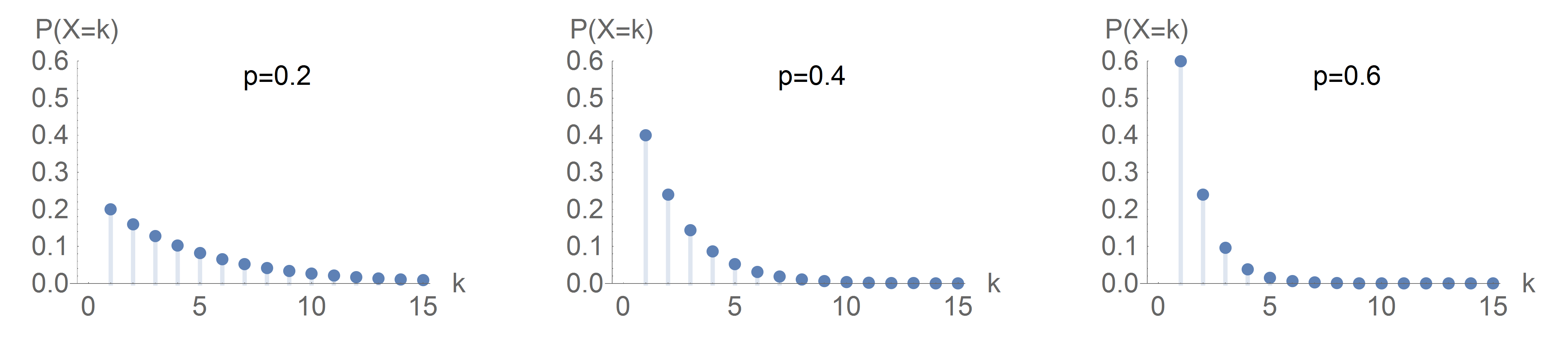
PMFs of the Shifted Geometric Distribution
Predictions, Outcomes, and Estimation
There are good arguments and evidence that during a simple Fishing World simulation, the total fishing effort of each fisher is independently drawn from a shifted-geometric distribution On average, it takes \(1/p\) casts to catch a fish. If the probability of success is \(p = 0.4\), on average it should take \(1/p=2.5\) tries to catch a fish. If the probability of success is \(p = 0.01\), on average it should take \(1/p=100\) tries to catch a fish. In addition, there can be considerable variability around this mean value. The variance is \((1-p)/p^2\); when \(p\) is small, this variance is large.
Estimation
The expected value of a probability distribution provides a natural prediction of the average outcome when sampling from the distribution. Of course, the sample mean is not typically an exact match to the predicted value. Nevertheless, the distribution mean provides a reasonable prediction of the sample mean.
Turning this around, one may estimate the underlying per-cast probability of success from the data. Suppose a researcher provides just the output data from a run of this model. Stipulating that each fisher samples from a geometric distribution with the same probability of success \(p\), what value of \(p\) seems most likely given the data?
Approach this question as follows. Label the uncertain end-of-simulation number of casts for each of \(N\) fishers as \(X_1, X_2, \dots, X_N\). Recall from the analysis above that, for any given \(p\), the probability mass function of the outcome \(X_i\) is the following.
Since each fisher’s outcome is independent of the other fishers, the probability of seeing the simulation’s entire actual set of outcomes (\(k_1,\dots,k_N\)) is correspondingly determined by the multiplication rule for independent events.
Given the data, call this expression the likelihood that the underlying probability is \(p\). This suggests an approach to estimating \(p\) from the data. Given the data, pick the value of \(p\) that makes this likelihood as big as possible. The result is the maximum likelihood estimate of \(p\).
As \(p\) goes from \(0\) to \(1\), the likelihood rises and then falls. This is easier to see by considering the logarithm of the likelihood, which turns multiplication into addition and exponentiation into multiplication.
Given the data, one may plot the resulting log-likelihood as a function of \(p\). Maximum likelihood estimation looks for the value of \(p\) that makes this as big as possible.
The differential calculus is an ideal tool for searching for the maximum-likelihood estimate; it can provide an analytical solution. If you are unfamiliar with differential calculus, skip the next step. Otherwise, find the slope of this log-likelihood function by differentiating with respect to \(p\). This yields the following expression of the slope.
The slope must be zero at an internal maximum, so set the slope expression to zero in order to characterize the most likely value of \(p\) (given the data). Simplify by multiplying by \(p(1-p)\).
Solve this equation for \(p\) to produce the maximum likelihood estimator for \(p\).
That is, the maximum-likelihood estimate the probability of success is the number of successes (\(N\), the number of fishes caught) divided by the total number of attempts (\(\sum_{i} X_i\), the total number of casts). This is just the multiplicative inverse of the mean number of casts.
Gather data from all the fishers at the end of a Fishing World simulation. Find the maximum-likelihood estimate of \(p\).
Likelihood Ratio Test
Recall that given \(p\), the probability that we would we see \(k_1, k_2, \dots, k_N\) is
We can compare the likelihood of seeing this outcome when \(p=0.01\) with the likelihood of seeing this outcome if it were actually the case that \(p = N/{\sum_{i} k_i}\). Call the former the restricted likelihood, \(L_r\). Call the latter the unrestricted maximum likelihood, \(L_u\). Naturally, the maximum likelihood must be the larger of the two.
Form the likelihood ratio \(L_r / L_u\). Since the restricted likelihood must be less than the unrestricted likelihood, it must be true that \(0 < L_r/L_u \le 1\). A value near \(0\) means that the restriction is very unlikely to characterize the data. A value near \(1\) means that the restriction is not very binding: the restricted likelihood is close to the maximum likelihood. This is the basis of a test known as the likelihood ratio test, based on this likelihood ratio.
As the number of observations becomes large, then minus the logarithm of the squared likelihood ratio approximates a chi-square distribution. This distribution has a single parameter, \(\kappa\), called the degrees of freedom. The degrees of freedom is the difference in the number of parameters in the restricted and unrestricted cases. In our application, \(\kappa=1\), since \(p\) is restricted when computing \(L_r\).
This test statistic has a value of \(0\) when \(L_r = L_u\). As \(L_r\) becomes relatively small, the logarithm of the likelihood ratio becomes very negative, and the test statistic correspondingly becomes large. Armed with \(\kappa\) degrees of freedom and a chosen level of significance, we can look up this test statistic in a chi-square table.
How unlikely is it that we would observe our simulation data \(k_1, k_2, \dots, k_N\) if the true value is \(p=0.01\)? For example, one simulation with \(1000\) fishers produced \(99,714\) casts producing an estimate of roughly \(p^*=0.01003\). In this case the ratio \(L_r/L_u\) is about \(0.996\). Look up \(\chi^2_1\) for \((-2 \ln[0.996])\) in a chi-square table, and find values at least this big happen frequently (more than 9 times out of 10). [2] Ordinarily we do not reject the null hypothesis unless we are quite unlikely to see a bigger test statistic (say, fewer than 5 times in 100 experiments). In this case, the test statistic under the null hypothesis that the two are equal is quite small, so we do not reject the null hypothesis. (And in fact, in this case, theory assures us \(p\) is the true value.)
A Controlling GUI for Fishing World
So far, this lecture has experimented with the model
by executing the runsim activity at the command line.
Previous lectures have emphasize that
GUI widgets often facilitate
initial experimentation with a model.
This section follows those earlier discussions quite closely,
reusing the GUI-building skills developed previously.
Model Parameters
Recall that we may conceptually distinguish the global variables, which change value as a simulation runs, from the model parameters, which do not. During a single simulation run, model parameters. may be considered to be global constants. Unfortunately, many languages will not allow you to request that, once set, the value associated with a name not be allowed to change. In such cases, the distinction between model parameters and global variables is informal: it is largely a matter of whether or not the value of a variable changes during a simulation run, not whether or not the programming language permits changing it. Furthermore, while model parameters are constant during one simulation run, we want to be able to alter focal parameters of different simulation runs. This is the basis of simulation experiments.
So far, the two key model parameters in a Fishing World are the number of agents and the fishing-success probability. Since this lecture explores the consequences of changing \(p\), it is the focal parameter. A focal parameter should have some baseline value, which may be arbitrary, but the computational implementation should make the actual value easy to vary.
How best to manage model parameters is a question
that this course returns repeatedly.
A good alternative is to introduce a name
that refers to the parameter value as needed in our program code.
That will be our approach:
we will introduce a global variable for each important model parameter.
For example, introduce a global variable named p,
initialized to \(0.01\),
for the fishing-success probability.
However, we also need a simple interface for changing this focal parameter.
name |
type |
value |
|---|---|---|
|
int |
1000 |
|
float |
0.01 |
Recall that the runsim activity consumes one argument—the
fishing-success probability.
(The runsim activity passes this to step activity,
which similarly requires one argument.)
Running a Fishing World simulation from the command line
required giving an argument to runsim (e.g., runsim 0.01).
This made it fairly simple to consider various values
of the focal model parameter.
Nevertheless, as in previous lectures,
it is convenient to move this focal parameter into a GUI slider.
Begin constructing a GUI for the FishingEconomy01 project
by creating a slider for p.
The possible values should be in \([0.01\,..\,1]\),
incrementing by \(0.01\).
(Running the simulation with a
success probability of \(0\) would produce an infinite loop.)
Set a default value of \(0.01\).
Exploratory Experimentation
For short-running simulations,
sliders and buttons enable easy interactive exploration.
This is particularly helpful early in the model-development process.
Such point-and-click exploration
can promote an intuitive understanding of the model
and even suggest changes to the model or new analyses.
As an initial example of such exploration,
this section consider the effect of p
on the running time of the simulation.
Iteration Tracking
Intuitively, with a larger fishing-success probability (p),
less time (fewer iterations) will pass until every fisher is fed.
To explore this,
prepare to record how long a Fishing World simulation runs
for various values of the model parameter p.
There are many possible approaches to this task.
For example, in the present model,
the number of iterations completed is the same as the
maximum value of nCasts among the fishers.
This section instead focuses on explicit tracking
the number of times the schedule is iterated,
as is common in discrete-time simulations.
To track the iterations,
introduce a new variable named ticks,
and initialize it to zero.
The ticks variable should increment
at the end of each iteration of our schedule.
Add a ticks variable to your model,
and modify the setup and step activities as follows.
The setup activity should intialize ticks to zero,
and the step activity should conclude by incrementing ticks
by one. For example, the step activity may now
be summarized as follows.
- activity:
step- parameter:
p: Real, the probability that a cast is successful- context:
global
- summary:
Update all fishers, and then increment the step counter.
Introduce a step counter.
Modify the step activity, as described above.
Note again that the step activity should
update all fishers only once.
Running-Time Experiment
After implementing iteration counting for this model,
we are ready to look at the response of running time
to the value of p.
This simulation experiment is particularly interesting because,
despite our knowledge of the distribution governing
the required effort for individual fishers,
we do not have a simple expression for the
maximum time spent fishing across our population of fishers.
[Margolin.Winokur-1967-JASA]
Even though a mathematical analysis of this problem is challenging,
an answer by means of simulation quite simple.
Set p to \(0.66\) and run the basic Fishing World
simulation a few times,
recording the final number of ticks for each run.
What is the mean duration of the simulation?
Repeat this process after setting p to \(0.33\).
What is the mean outcome?
Do the results match your intuition about the effect of changing p?
Optional: Set up this experiment more formally. Let \(p\) take on values from \(0.1\) to \(1.0\), stepping by \(0.1\). For each value of \(p\), run the Fishing World simulation \(100\) times. Collect the number of iterations from each run. Plot the mean number of iteration against \(p\). Separately, plot the variance of the final number of iterations against \(p\).
The Evolution of Hunger
Some fishers stop fishing early in the day, while others must continue fishing to catch a fish. During each execution of the simulation schedule, only the hungry fish.
A Day in a Village
In a basic Fishing World, fishing and eating constitute a day in the life of the villagers. As the day progresses, more and more fishers are successful and are able to eat. A useful summary of the state of the village is the number of fishers who are still hungry. At each simulation step, this number cannot increase, and over time it gradually declines. It is possible to track this evolution of the system state during an entire day. That is, each core simulation step, we can record the number of hungry fishers.
Count Hungry Fishers
In a Fishing World,
it is simple to determine the number of hungry fishers.
Simply count up all the fishers with
a value of 0 for the nEaten attribute.
This describes a countHungry function,
as in the following function sketch.
- function:
countHungry: Set[Fisher] -> Integer- function expression:
\(\mathrm{fishers} \mapsto {}^\#\{f\in\mathrm{fishers} \mid \mathrm{isHungry}[f]\}\)
- parameter:
\(\mathrm{fishers}\), the set of fishers
- summary:
Return the number of fishers who are hungry.
Implement the countHungry function.
(You may optionally support it with a separate isHungry function.)
Confirm that it returns \(1000\) immediately after the setup phase
and \(0\) after a Fishing World simulation completes.
Optionally, implement a more formal test.
Dynamically Monitor a Fishing World
When a simulation takes some time to run, it can sometimes be useful to dynamically monitor key outcomes as it progresses. For implementations in some languages on common hardware choices, Fishing World simulations may run too quickly for dynamic monitoring to be useful. In such cases, a post-simulation plot of the data is generally more useful. (See below.) Nevertheless, this section considers dynamic monitoring of the evolution of hunger. The focus will be the proportion hungry at the end of each iteration.
The simplest way to dynamically monitor this value is to simply print it out at the end of each iteration. However, simulation toolkits often provide facilities for the creation of dynamic GUI monitors, and these can be a useful part of a simulation-model GUI during the early stages of experimentation. So another way to dynamically monitor this value is to create a GUI monitor that continually reports the proportion of fishers who are still hungry.
Optional:
Add dynamic monitoring of the proportion hungry
to the FishingEconomy01 project.
(Utilize the countHungry function.)
You may simply print out the value after each simulation step.
However, if you are using a simulation toolkit that easily supports it,
add a dynamic monitor to the FishingEconomy01 GUI.
This monitor should display the proportion of fishers still hungry,
updating after each simulation step.
Optional: Additionally add a dynamic monitor for the mean number of casts of the fishers and the end of each core simulation step.
Collect the Hunger Data
The next task is to collect the hunger data by writing it to a file. The file should have a CSV format, to ensure that the exported data can be opened by any spreadsheet or statistical application. The data accumulates as the simulation runs, so there are two basic choices for export: either collect the data in memory for an end-of simulation bulk export, or export it incrementally after each core simulation step. This section focuses on incremental export, but either approach is fine.
Let a recordStep activity describe incremental export,
which exports data at the end of each iteration.
For the FishingEconomy01 project, after each core simulation step,
export two numbers to a new line:
the value of ticks,
and the proportion of hungry fishers.
(Use countHungry to compute the number of hungry fishers.)
These should be separated by a comma
and appended to the output file,
so that the final result is in CSV format.
Name the output file fishingSurvival.csv,
and remember always to export your data to your designated output folder.
- activity:
recordStep- context:
global
- summary:
To your designated output file, append a record of the current model state.
Export a time series of the model state
to a fishingSurvival.csv file in your designated output folder.
Each line of the file should hold the current value of ticks
and the current proportion of fishers who are hungry
(separated by a comma).
Use the countHungry function to help compute the proportion hungry.
To perform the data export incrementally,
implement a recordStep activity
that appends a single CSV line to fishingSurvival.csv.
Then modify the runsim activity
to execute this recordStep activity
in order to record the data after each core simulation step.
Also, modify the setup activity to initialize
the fishingSurvival.csv file:
write a header and an initial line of data:
the initial value of ticks (\(0\)),
and the initial proportion hungry (\(1.0\)).
(You may wish to implement a separate setupOutputFiles activity
that discards any old data, writes the header, and records the initial state.
Simulation Schedule Redux
With incremental data export and dynamic monitoring,
the simulation schedule during the iteration phase
now includes more than the core simulation step.
Rather than modify the step activity,
it is common to create an encompassing activity.
For example, we can implement a go activity
that executes the core simulation step,
then records the data,
and finally performs any needed GUI updates.
- activity:
go- context:
global
- summary:
Execute the core simulation step.
Update the per-iteration output file (i.e., export the data from this iteration).
Update the GUI as needed.

Simulation Schedule
Survival Function
Recording the number hungry relative to the original population produces an empirical survival function. Recall that for a random variable \(X\), the survival function \(S[t]\) gives the probability of an outcome greater than \(t\).
In Fishing World, consider the probability that it will take more than \(t\) casts to catch a fish. Each hungry fisher casts once each iteration, so the survival function states the expected proportion of fishers who are still hungry after \(t\) iterations. Here for example are some theoretical survival functions for shifted geometric distributions with various success probabilities.
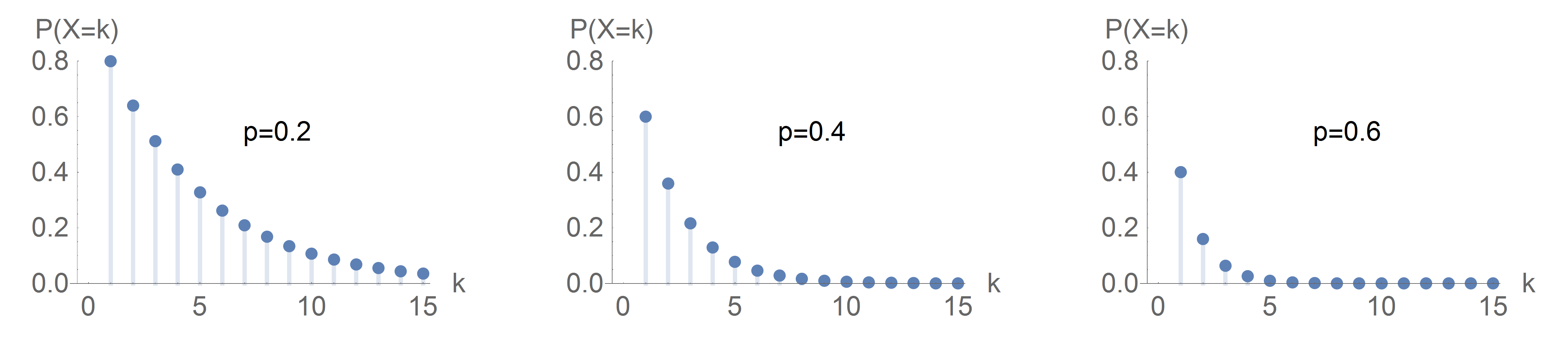
Survival Functions of Shifted Geometric Distributions
Simulation Results
Modify the runsim activity
to execute the go activity.
Set p to 0.01
and run the model until no fishers are hungry.
An empirical survivial plot show the proportion still hungry
after each core simulation step.
Import the hunger data into a spreadsheet and create an empirical survival plot,
which you should save as fishingSurvival.png.
Optional: Add a time-series line chart to the FishingEconomy01b project’s GUI. This should show the proportion of fishers who are hungry over time.
With 100 fishers and a 0.01 chance of success each cast,
we may get a result like the following.
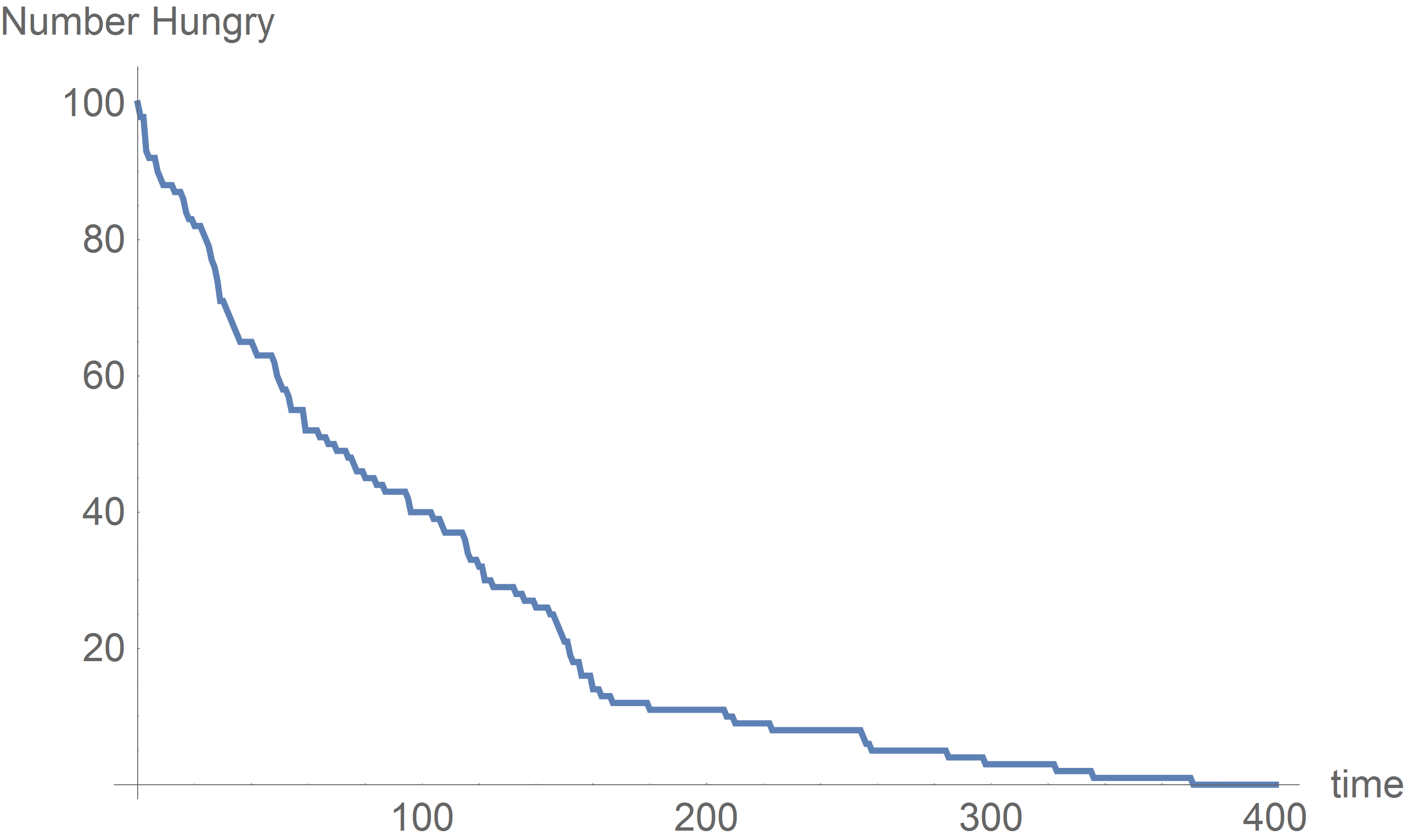
One Village Day: nFishers=100, p=0.01
Interpreting the vertical scale of this plot as a percentage, this plot presents an empirical survival function. Compare this to a theoretical survival function.
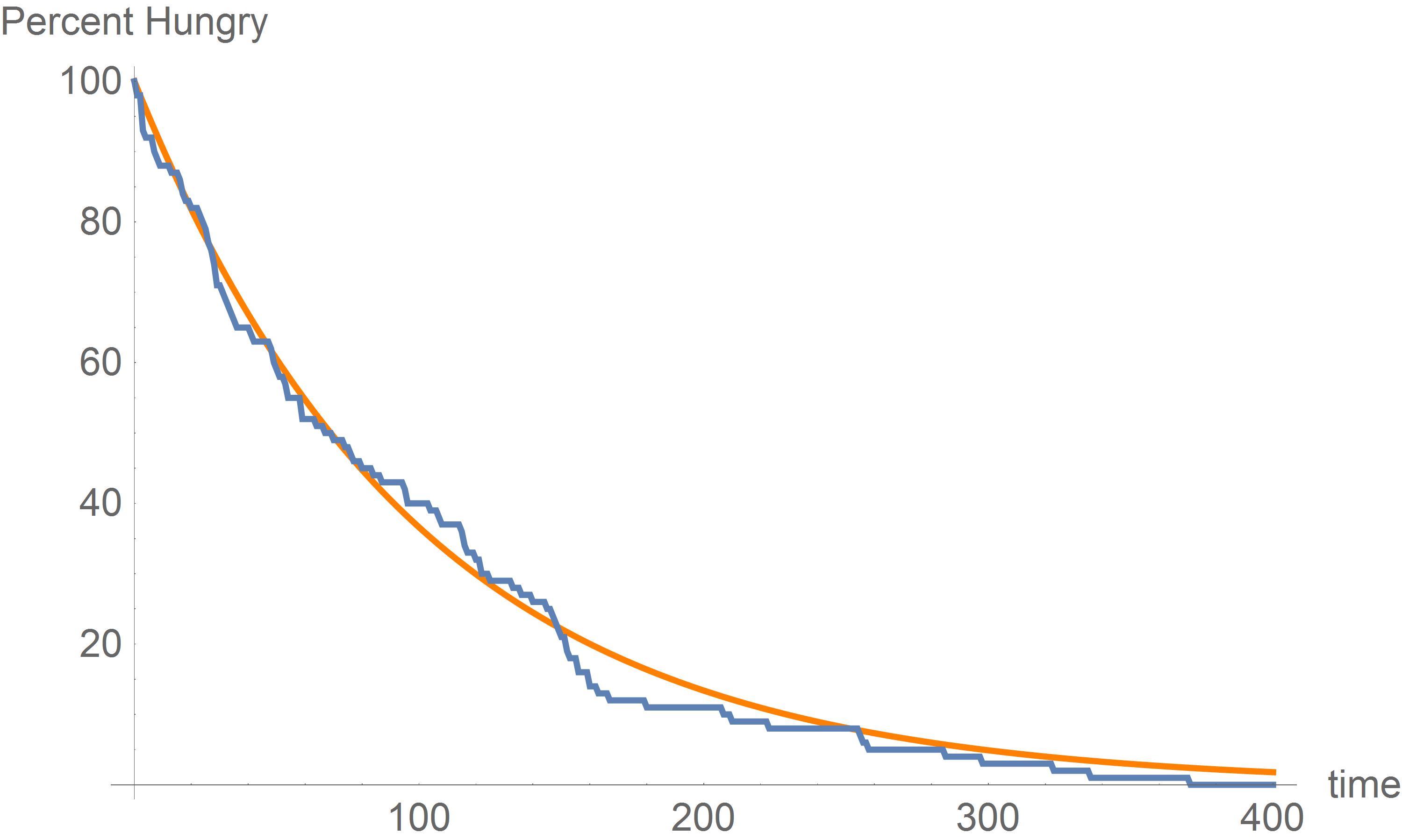
Theoretical vs Empirical Survival Function
Finite Workday
Fishing may go on a long time before succeeding. So far we have assumed that a hungry fisher keeps fishing. Now we allow that the workday is of finite length. A fisher who has not caught anything by the end of the day goes home hungry.
Workday of a Fisher
Measure the length of the workday in fishing attempts.
Call the length of the workday nMaxCasts.
This is a new model parameter.
The likelihood of going home hungry depends on the length of the workday and the ease of catching fish. (It does not depend on personal characteristics, because all fishers are equally skilled, and all face a common workday.)
Given a finite workday,
how many fishers go home hungry?
This is random:
on some days many fishers are lucky,
while on other days many fishers are unlucky.
Both the fishing probability (p)
and the length of the day (nMaxCasts)
affect the number of fishers that go hungry.
It is possible to make a prediction, as follows. Calculate the probability that any single fisher goes hungry: \(P[X > \mathrm{nMaxCasts}]\). This may be easier to compute as \(1 - P[X \le \mathrm{nMaxCasts}]\). (That is, the complement of the probability of catching a fish in time.) The expected proportion fed (\(f\)) is:
which implies that
Together these imply that
For example, if p = 0.01 and nMaxCasts = 400
we get \(f \approx 0.98\),
so on average 98% of fishers will eat each day.
The corresponding expected proportion hungry is \((1-f)\),
or around 2%.
Fishing World: Stopping Condition Redux
As part of our simulation, we need to decide how long the simulation will run. That is up to us, as creators of the model. In the simplest case, Fishing continues as long as there are any hungry fishers. If we decide that it is more realistic to impose a finite day, fishing continues until the day ends.
- activity:
go- context:
global
- summary:
If the day has ended, stop.
If nobody is hungry, stop.
Update all fishers (in random order).
Update all global variables (i.e., increment
ticks).Update the output file (i.e., export the data from this iteration).
Update the GUI.
Location of the Stopping Condition
If our Go button simply executes the current step activity,
then (since it is a forever button) activating the button
will cause the simulation to continue to run even after
all fisher have eaten.
There are two salient possibilities
for incorporating the stopping condition in this situation.
The first is to include the stopping condition in the button code.
The second is to move the stopping condition into the step procedure.
Neither choice is inherently superior,
but the latter is more visible to someone examining the code.
In this course, we consider that enough of an advantage to determine the choice.
If we test for the stopping condition at the very beginning of the step procedure,
this approach has another feature that we will consider advantageous.
With this arrangement,
executing the go procedure will not produce any additional iterations
once we have satisfied the stopping condition.
With this decision, we must modify our step activity.
- activity:
go- context:
global
- summary:
If nobody is hungry, stop.
Update all fishers by calling
step.
For example, your could put the following code at the very beginning of
your go activity.
if (all? fishers [1 <= nEaten]) [stop]
Update your go activity to begin by testing a stopping condition.
(We will make further modifications later on.)
Simulation Results with Finite Work Day
Here we report the results of a few simulations. Of course the number who go hungry in any particular simulation differs randomly from the number expected.
nFishers |
p |
nMaxCasts |
number hungry |
expected hungry |
|---|---|---|---|---|
1000 |
0.60 |
4 |
21 |
26 |
1000 |
0.60 |
4 |
32 |
26 |
1000 |
0.01 |
4 |
961 |
961 |
1000 |
0.01 |
4 |
953 |
961 |
1000 |
0.01 |
400 |
12 |
18 |
1000 |
0.01 |
400 |
23 |
18 |
Naturally, more go hungry if the probability of catching fish is lower or the length of the day is shorter.
Summary and Conclusions
Exploration, Resources, and References
The following explorations are not part of the assignment!
Fishing World Explorations
Add a button to export the fishing-effort data. (Optionally: disable the button until the end of a simulation.)
Consider the first absolute-frequency plot in this lecture. What happens if you change to a ratio scale for the counts?
Do the Fishing World results depend on the number of fishers? (Add a slider for easy experimentation.)
Colorful Agents:
We would like to be able to monitor the progress of our simulation. Our first approach to this will be to color code our agents. Color the fishers red when hungry and green when not.
NetLogo-Specific Explorations
For the basic Fishing World, confirm that the following version of
updateFisherimplements the conceptual model.to updateFisher01 [#p] if (1 > nEaten) [fish #p] if (canEat) [eat] end
For the basic Fishing World, an alternative implementation of
updateFisherimmediately exits the activity when a fisher is not hungry. Achieve this in NetLogo by combining anifelsestatement with thestopcommand, as follows.to updateFisher02 [#p] ;fisher proc ifelse (1 > nEaten) [fish #p] [stop] if (canEat) [eat] end
Confirm that this version of
updateFisheralso implements the conceptual model.This approach produces two separate points of exit from the activity: where
stopoccurs, and whereendoccurs. Programmers sometimes debate the wisdom of allowing multiple points of exit from an activity. This course considers early exit to be a fine practice as long as it makes the code easier to understand.
Resources
Geometric Distribution
Most textbooks on probability and many introductory textbooks on statistics include a discussion of the geometric distribution. The free online textbook by [Illowsky.Dean-2022-OpenStax] offers a brief and intuitive introduction. The advanced discussion by [Margolin.Winokur-1967-JASA] covers details about the distributions of order statistics.
Bin Probabilities of a Geometric Distribution
Geometric distributions have many nice properties, one of which is the constant ratio of adjacent bin probabilities. To see this, bin together adjacent values from a geometric distribution. For example, create bins of width 3, and consider the probabilities of falling in either of two adjacent bins.
The ratio of the latter probability to the former is \((1-p)^3\). This does not depend on the value of \(k\). In other words, the odds of adjacent bins again have a constant-ratio property. This property depends only on the adjacent bins being of equal width.
NetLogo-Specific Resources
To test whether any fishers are still hungry, One might test whether
any? fishers with [0 = nEaten]. However, thewithoperator constructs a new agentset by testing every agent. Instead, one might test whethernot all? fishers [1 <= nEaten]This will not construct a new agentset. Furthermoreall?returnsFalseas soon as it encounters a hungry fisher. (This is called short-circuit evaluation.) For this reason, one may prefer to useall?, especially if the number of agents is large.Instead of
while, one may use theloopprimitive. (Review the syntax forloopin the NetLogo Dictionary and in the NetLogo Programming supplement.) Theloopcommand starts an infinite loop, but thestopcommand breaks out of this loop. Here is the same simulation usingloop. (Just enter the code at the NetLogo command line.)setup loop [if (all? fishers [1 <= nEaten]) [stop] step]
NetLogo’s
loopcommand is a bit unusual: most programming languages do not include its equivalent. Across languages, the much more common looping construct iswhile. When an explicit indeterminate loop is required, this course will generally favor the more traditionalwhileconstruct. Note that theloopexample uses the stopping criterion directly, whereaswhileuses its negation.One might be tempted to simplify by putting the stopping condition inside the
stepactivity. Howeverloopis not designed to detect whether a activity that it calls has executedstop. (In contrast, forever buttons are so designed.)
References
Downey, Allen B. (2015) Think Python: How to Think Like a Computer Scientist. Needham, MA: Green Tea Press. https://greenteapress.com/wp/think-python-2e/
Illowsky, Barbara, and Susan Dean. (2022) Introductory Statistics. : OpenStax. https://openstax.org/details/books/introductory-statistics
Margolin, Barry H., and Herbert S. Winokur. (1967) Exact Moments of the Order Statistics of the Geometric Distribution and their Relation to Inverse Sampling and Reliability of Redundant Systems. Journal of the American Statistical Association 62, 915--925. http://www.jstor.org/stable/2283679
Copyright © 2016–2025 Alan G. Isaac. All rights reserved.
- version:
2025-07-14