Multi-Agent Modeling and Simulation
- Author:
Alan G. Isaac
- Organization:
Department of Economics, American University
- Contact:
- Date:
2024-05-15
Overview and Objectives
Overview
Goals and Outcomes
This lecture continues our exploration of multi-agent modeling and simulation. It also explores some core agent-based modeling issues in a tentative way, with the understanding that later lectures will add detail and depth. Central to the present lecture is the complete development of a very simple multi-agent model of wealth distribution.
Prerequisites
This lecture presumes prior mastery of the material in the Logistic Growth lecture. This is particularly true of the exercises.
The exercises of this lecture presume the mastery of certain preliminary material. Before attempting them, be sure to read the Exponential Growth lecture. Additionally, carefully read the the discussion of model parameters in the Glossary to this course.
For the data analysis of this lecture, certain basic spreadsheet skills are needed. These are covered in the Spreadsheet Introduction supplement. Do the following spreadsheet exercises: Step Chart and Frequency Chart.
MAMS: The Process of Programming
Before attempting order to implement the model below, skim this lecture from start to finish. Be sure to garner a good sense of the conceptual model and of the charts of the model results. Then work through the lecture step by step, implementing the computational model as you go. Keep the implementation runable by temporarily using stubs during model development. Verify the implementation of functions, either by using provided test procedures or by writing your own.
Agents
Focus on the Actors
As we saw in the Financial Accumulation lecture, multi-agent simulation models explicitly represent individual actors. These actors models are called agents. This lecture again shows that the idiosyncratic histories of initially identical agents produce not just divergent individual outcomes but also systemic regularities.
Minimal Agent
Attributes
This lecture again works with a minimal agent.
A wealth stores an agent’s wealth as a real number.
The Risks of Mutable State
Agent-based models are often implemented with mutable agents.
One tricky thing about this is that a program may have
more than one reference to an agent whose state can change.
For example, if variables x and y refer to the
same agent and a procedure changes the wealth of y,
then of course the wealth of x also changes.
Or, if in a list of agents one of the agents changes its wealth,
then even though the list contains the “same” agents
the list is no longer in the same state.
A certain lack of transparency is created by working with objects that have mutable state. It means that it can be difficult to predict the output of functions that use these objects as inputs. As a simplest example, suppose the input to a function is a mutable agent. Even if the function does no more than return the wealth of that agent, predicting the value that will be returned is problematic, since the wealth may change as the program runs. Prediction requires not only knowledge of which agent is input but additionally the current state of that agent. This loss of transparency is a definite cost to the approach. Offsetting this, mutable agents often provide a very natural way to think about behavior.
User-Defined Attributes
A conceptual model of a type of agent specifies the data each agent owns and the behaviors of which it is capable. These are the key decisions in agent design.
For example,
consider the design of a type of gambler agent.
Think of a gambler as owning a certain amount of wealth.
This suggests that a gambler has a wealth attribute.
In a simple model,
the current wealth of a gambler may constitute its current state.
Next, turn to behavior.
Presumably, a gambler is able to gamble.
The conceptual model of the gambler type may therefore include
a bet behavioral attribute.
In this lecture,
a gambler is able to wealth to place bets.
Betting behavior leads to changes in the gambler’s state
(i.e., in current wealth).
Classifier Diagram: Minimal Agent with Wealth
In order to better conceptualize and communicate this conceptual designs, modelers often rely on visual aids. A popular chart for agent design is the UML classifier diagram. For example, summarize the proposed design of a gambler agent with the following visual representation.
wealth: Integer = 100 |
bet(amt: Integer) |
Recall that the rectangle is a UML classifier symbol, and it is broken into three compartments. The first compartment holds the name assigned to this agent type. The second compartment lists the attributes, possibly along with the data type of each attribute. Behaviors are listed in the third compartment, with any parameters listed within appended parentheses. [1]
In this particular case, there is only one attribute, and one behavior. The classifier diagram specifies that the wealth attribute is assigned integer values, wih a default initialization of \(100\). Such additional detail is optional but can often be useful.
For each attribute,
a class box diagram may provide a data type and an initial value.
Saying that wealth has a Real type essentially means that it is an
ordinary real number, which can take on any fractional value.
(The representation of such numbers varies by computer language.)
The initial value of \(1.0\) for the wealth attributed
is a fairly arbitrary starting point used in the simulations below.
Recall from the Financial Accumulation lecture that parentheses are appended to behavior names in the class box, but that these parentheses are purely a visual aid (to help distinguish behaviors from data attributes).
Although the diagram tells us that the wealth attribute has takes on integer values, it fails to specify the units. This lecture works with an extremely abstract agent, and corresponding currency unit is artificial. The scarab, represented by the ¤ character, is an international symbol for an unspecified currency unit.
Agents: Conceptualization vs Implementation
There are tools for some object-oriented programming languages that can translate detailed class diagrams rather into implementations in code. In that case, diagrams can become formal representations of the actual code that implements an agent. In contrast, this course uses such diagrams simply to guide model conceptualization. A given diagram can be given many different implementations in code.
For example, the classifier diagram of a Gambler
just specifies the attributes and behaviors of a conceptual gambler.
It is not meant to imply any particular approach
to representing these attributes and behavior in code. [2]
To drive this distinction home,
this section develops a gambling simulation
without defining any Gambler type.
Behavioral Details
Nevertheless, much more behavioral detail is needed before
a conceptual model can lead to an implementation in code.
A Gambler has a betting behavior,
but what does betting look like?
The conceptual model remains radically incomplete until
it provides the details of this behavior.
In this lecture,
a Gambler will place a bet of 1,
which will either be forfeit or doubled,
with equal probability.
However, we will
As a consequence of betting once,
the wealth of a Gambler can either increase by \(1\) or decrease by \(1\).
Behavior has consequences:
it changes the state of the agent.
Aggregation into Collectives
Choosing the appropriate level of aggregation is often an important decision in computational modeling. As suggested by the list of possible agents, some agents in a conceptual model may represent groups of component agents. Sometimes we make this explicit, so that collective agents explicitly comprise component agents. For example, a firm may comprise many workers. In this case, the question of whether a firm is anything more than its component agents becomes interesting. Later lectures explore situations where a collective agent both comprises other agents and has its own separate actions.
A Single-Agent Gambling Simulation
The section works with the conceptual model of a Gambler
that Figure f:basicGambler presents.
One goal is to develop an implementation in code
of this conceptual description of the Gambler agent type.
A second goal is to reuse many of the tools and concepts from
previous lectures to create
a very simple single-player simulation model based on this agent type.

Simple Gambler
User-Defined Attributes and Behaviors
A Gambler has a wealth attribute,
with an initial value of \(100\),
and a bet behavior.
Therefore, any computational implementation of the gambling model
must somehow endow a gambler with a wealth attribute
and a bet behavior.
However, the best approach to these needs is extremely language dependent.
This course assumes the use of a language where there is a fairly obvious way to create individual agents with user-defined named attributes. It also assumes the language provides an easy way to associate behaviors with these agents. Later sections make extensive use of these facilities.
User-Defined Behaviors
The single-gambler model of this section has a single gambler
with a wealth attribute and a bet behavior.
The are many ways to approach a computational implementation
of the conceptual model.
Nevertheless, any computational implementation of the gambler model
needs not only to create a wealth endowed agent,
it must also provide a way for this agent to engage in betting behavior.
We therefore need a way to add user-defined behaviors.
Random Behavioral Consequences
Behavior has consequences. Often, those consequences are not completely predictable. Instead, there is some randomness in the outcome. Outcome uncertainty is an important consideration in real world behaviors, and agent-based modeling readily accommodates such uncertainty.
Gambling
A Gambler can place a bet that, with equal probability,
is either be forfeit or doubled.
In the present model, a Gambler always bets ¤1
(one monetary unit).
The possible changes in wealth due a single bet are correspondingly
an increment of 1 or a decrement of 1.
The ways to produce these random outcomes is language-specific.
This section assumes that the implementation language
provides facilities for random choice from a sequence.
This sequence will be hardcoded in the bet procedure.
- procedure:
bet- parameter:
amt- context:
Gambler- summary:
Let
paritybe \(1\) or \(-1\), with equal probability.Change
wealthbyparity * amt.
Implement a
betprocedure as described above.Implement a
testBetprocedure that tests that thebetprocedure works as expected.
Setting Up the Model
Recall that this course follows the convention that
a setup procedure performs the model setup.
Model setup includes setting the values of model parameters
and initializing any global variables.
For convenience,
let the computational model include a global variable name ticks,
conventionally used to track the number of model iterations.
It also includes any initial agent creation
and intialization of the agents.
In the single-gambler gambling model,
the setup procedure may resemble the following.
- procedure:
setup- context:
global
- summary:
Create a
Gambleragent.Initialize the agent’s
wealthattribute to100.Set
ticksto0.
Model setup is just the initialization of
the gambler’s wealth attribute and the global ticks variable.
After implementing the setup and bet procedures,
run a single this simulation step by executing setup
and then executing bet.
This simulates the outcomes of one gambler placing one bet.
After running this simulation,
examine the final state of the agent.
(That is, print the value of wealth.)
Implementing the Gambler
Perhaps the simplest imaginable gambling simulation sets up one gambler and then considers a single betting action.
Create a project file named
"Gambler00"(plus an appropriate filename extension).Give your gambler a
wealthattribute.
Implement a
setupprocedure that setswealthto 100 andticksto0.
Creating a testBet procedure poses a new challenge.
Starting with a wealth of \(100\),
executing bet 1 produces a wealth
of either \(99\) or \(101\).
The result is random.
One approach to the problem is to insist
that wealth be either \(99\) or \(101\).
This can be achieved by testing for satisfaction
of a logical disjunction.
Implementing the Gambler (NetLogo Details)
NetLogo provides the one-of reporter;
when applied to a list of numbers,
it returns a random choice from the list.
This meets the needs of the gambling model.
If necessary, review the
introduction to lists
in the Introduction to NetLogo supplement.)
Then use the list primitive
to can create the list of outcomes as follows.
(list -1 1)
To illustrate picking a random member from our list of possible outcomes, enter the following multiple times at the command line:
one-of (list -1 1)
Sometimes the result is -1;
sometimes the result is 1.
This provides a simple representation of random outcomes.
Each application of the one-of reporter to the same list
may produce a different value.
As mentioned above,
this creates a new challenge for testing.
Here is one simple approach to testing the bet procedure.
to testBet
  setup
  if (100 != wealth) [error "bad setup"]
  bet 1
  if not (99 = wealth or 101 = wealth) [error "bad bet"]
  print "testBet passed"
end
Single-Gambler Simulation: Simulation Schedule
Recall that a typcial simulation specifies a schedule:
a sequence of actions that repeatedly executes as the simulation runs.
The schedule should be written so that it provides
an easily understood outline of the steps followed
in the simulation.
This includes a specification of
which agents are acting in which order, and what they are doing.
Currently we have only one agent, the single Gambler,
who has one behavior, bet.
The single-gambler simulation has a very
simple simulation schedule.
The model step comprises a single betting action,
which changes the value of wealth,
and an export the value of wealth to the
file "out/gamblerWealth00.csv".
We chose the name step for the procedure specifying
the simulation schedule.
The name go is somewhat more conventional in NetLogo programming,
but it is less descriptive.
When implementing our model of a gambler,
the step procedure contains the following schedule.
- procedure:
step- context:
global
- summary:
The gambler places a bet of \(1\).
Write the new value of
wealthto the output file.
The simulation is correspondingly simple.
Setup the simulation model,
and then execute the step procedure \(100\) times.
For convenience,
create a runsim procedure that runs this simulation.
- procedure:
runsim- context:
global
- summary:
Setup the model.
Run \(100\) iterations of
step.
Implement a
stepprocedure that comprises a single bet (of \(1\)) and an export of wealth to the output file,"out/gamblerWealth00.csv".Implement a
runsimprocedure that callssetupGlobalsand then callsbet(1)a total of \(100\) times.
NetLogo: Simplest Gambling Simulation
Enter the following at the NetLogo command line.
setup
step
This runs our simples gambling simulation.
Afterwards, we might use the print command
to examine the final state of our agent.
print wealth
Iterating a Schedule
There are a few ways in which our simplest gambling simulation is too simple. Here we address one of them. In a typical simulation, the simulation schedule exectues repeatedly. One repetition of the schedule of actions is called a step or an iteration. When this schedule is repeatedly executed, we say it is iterated. An iteration typically changes the state of the program in some way, and the new state serves as the starting point for the next iteration.
In our gambling model, there is a single schedled action: the gambler bets. Our schedule is correspondingly simple: it comprises this single action. As this schedule iterates, the gambler bets repeatedly.
Looping Constructs
A typical simulation involves not just one
but many iterations of the schedule.
(The question of how many can be very important,
and we will return to it.)
Suppose we want to execute \(100\) iterations of the schedule.
Even though the name step is very short,
we do not want to enter it \(100\) times at the command prompt.
Instead we rely on a looping construct. Looping constructs are designed to allow us to easily execute a code block a large number of times. Looping is a core programming concept.
There are two basic types of loop:
determinate and indeterminate.
Determinate loops execute a fixed number of times,
independently of what happens in the loop body.
Indeterminate loops execute a number of times
that depends on what happens in the loop body.
Let us first consider a simple determinate loop,
which executes the step procedure \(100\) times.
NetLogo Looping: repeat
The simplest NetLogo looping construct is repeat,
which implements a determinate loop.
The repeat command takes two arguments,
a number of repetitions,
and a command block to execute repeatedly.
We could represent this as:
repeat <number> [<commands>]
As always, angle brackets indicate where substitutions are needed. To illustrate, enter the following at the command line.
setup
repeat 100 [step]
print wealth
Outcomes
Printing the final wealth of the gambler offers one perspective on the simulation results. Another perspective emerges if we plot the value of wealth over time. (We explore this in more detail, below.)
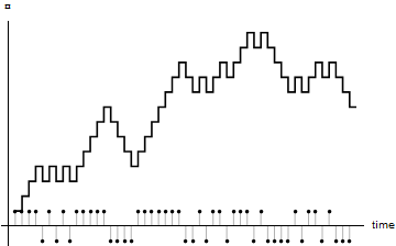
Simple Gambler’s Wealth over Time
Multi-Gambler Simulation
This section develops a multi-agent gambling model.
Each conceptual agent in the model is a Gambler.
Multiple Agents
One way in which the simplest gambling model is too simple is that it includes only a single agent. A model with a single agent is not generally considered to be “agent-based”. Typically an agent-based model will involve scores or even thousands of inidividual agents. The project of this section is therefore to produce a simulation model with many gamblers.
To fully specify a simulation we need to specify the number of agents. For now, use \(1089\) agents. Depending on the language we choose for our simulations, we may collect our gamblers together in some kind of set-like or list-like data structure.
Many Gamblers
To produce a model of many gamblers,
make the following changes.
The setup now needs to set up all the gamblers,
and step procedure must cause each gambler to bet.
To run the multi-agent simulation, proceed as before:
run the setup procedure,
and then run the step procedure \(100\) times.
Setting Up the Multi-Gambler Simulation
This course follows the convention that
a setup procedure performs the model setup.
Model setup includes setting the values of model parameters
and initializing any global variables.
It also includes any initial agent creation
and intialization of the agents.
In multi-gambler gambling model with \(1089\) agents,
the setup procedure may resemble the following.
- procedure:
setup- context:
global
- summary:
Create \(1089\)
Gambleragents.Initialize each agent’s
wealthattribute to100.Initialize
ticksto0.
Simulation Outcome
After running the simulation with many gamblers, we need to look for ways to characterize the final outcome. A first thing to try is simply printing the wealth values for all our gamblers.
Summarizing the Outcomes: Frequencies
Unfortunately, printing the value of the wealth attribute
for so many agents produces a lot of data,
and it can be hard to detect useful patterns in a printed collection of numbers.
The resulting list of a numbers does not appear
particularly informative about our multi-agent simulation.
In upcoming lectures, we will repeatedly return to questions about how best to produce and summarize data to characterize our simulation outcomes. For the moment, let us simply produce the mean and variance of the outcomes. (These statistical concepts are reviewed in the Basic Statistics supplement.)
Prediction: Micro vs Macro
The results of our computational simulation and of the Galton board simulation suggests that although individual outcomes are quite unpredictable, the aggregate outcomes reliably display patterns. This is an example of the emergence of predictable macro (i.e., aggregate) outcomes from unpredictable micro (i.e., individual-level behaviors). This provides our first suggestion that multi-agent simulations may be more useful in predicting macro patterns than micro outcomes.
Coleman’s Boat
Figure f:boatColeman shows a common representation of macro-micro linkages, widely known as Coleman’s boat and frequently attributed to [Coleman-1986-AmJSoc]. This diagram is a heuristic aid to thinking about causal relations between sociological (“macro”) facts. While it is tempting to posit direct causal linkages between macro-level preconditions and macro-level outcomes (see arrow 4), Coleman argued that a more careful theoretical analysis must encompass (micro-level) individual perceptions and behaviors. The postulated link between macro-level conditions and outcomes is represented by arrow 4. However, this is intermediated by the causal links between micro-level conditions (e.g., perceptions) and outcomes (e.g., actions), represented by arrow 2. Arrow 1 indicates that macro-level conditions (e.g., a normative environment, or current market prices) affect individual perceptions and beliefs. Arrow 3 indicates that, somehow, individual actions aggregate to macro-level outcomes. Arrow 3 does not represent a simple average of individual outcomes, but rather it represents a possibly complex transformation rule that governs the relationship between individual actions and measurable social outcomes. For example, the relationship between individual home-buying strategies and emergent measurable neighborhood segregation may be difficult to capture without a simulation model.
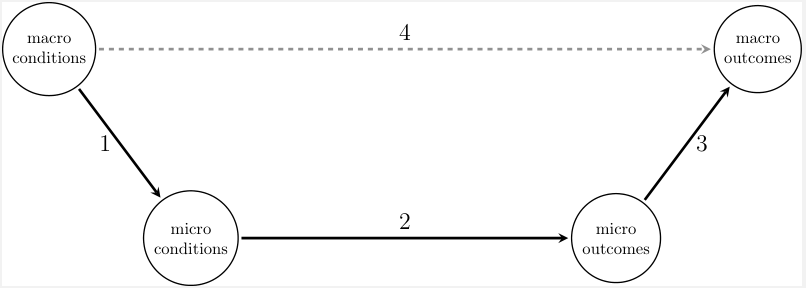
Coleman's Boat
A traditional representation of macro-micro linkages. (Adapted from Figure 1 of [Raub.Buskens.VanAssen-2011-JMathSoc].)
Multi-Gambler Simulation: A Physical Implementation
Recall the conceptual model of a gambler. A gambler faces equal probability of losing or gaining ¤1 with each gamble. When we consider many gamblers, they gamble completely independently, with no interaction between gamblers. Based on this conceptual model, we developed a simulation model, implemented in software.
Now imagine a physical implementation of a simulation, based on a Galton board. A Galton board typically implemented an inclined wooden board with nails arranged in offset rows so that a ball gently rolled down the center of the board has and equal likelihood of shifting one column to the left or to the right each time it descends by a row. (The Galton board is sometimes called a quincux, based on the simlarity to the arrangement of dots for the number \(5\) on a standard six-sided die. Less reverently, it is sometimes called a bean machine.) Balls are collected in bins at the bottom or the board, in order to record their final positions. Before reading further, view a video of a Galton board in action. (Many are available on the Internet.)
A Physical Gambling Simulation
To simulate the outcomes for a single gambler who gambles \(t\) times, we simply let a marble roll through the Galton board with \(t\) rows, starting at the center. Interpret a bounce to the left as a loss of ¤1 and a bounce to the left as a win of ¤1. The final change in wealth is the final distance from the center. To simulate the outcomes for many gamblers, we let many marbles sequentially roll through the board, each starting at the center.
This implementation differs slightly from our computational implementation, when it comes to the sequencing of gambles. In the computational model, every gambler gambles once, and then every gambler gambles again. In the physical model, the first gambler gambles \(t\) times, and then the next gambler gambles \(t\) times. (Although we can allow multiple marbles rolling through the board at the same time, as long as they enter sequentially.) This difference does not affect our simulation outcomes, since the outcome of each gamble is completely independent of all other gambles. Although characteristic of this gambling model, the irrelevance of sequencing is not generally characteristic of simulation models.
NetLogo: Galton Board Simulation
The NetLogo models library includes a simulation of a Galton board. Get the Galton Box model from the NetLogo Models Library, and experiment with it. Start with a single ball, and run a few simulations while looking for a patterns in the outcomes. Then increase the number of balls to \(100\), and run the simulation again. Now it should be easy to see the tendency of the simulated balls to land near the center, producing the roughly bell-shaped aggregate outcome that you should have observed in an online video.
Multi-Gambler Simulation: NetLogo Details
NetLogo Agentsets
In NetLogo, we often work with a set-like
collection called an agentset.
An agentset is an unordered collection of agents.
For the present project,
let patches as the agents.
NetLogo automatically provides a builtin patches primitive
that reports an agentset containing all the patches.
By default, NetLogo provides \(1089\) agents
(identified by locations on a \(33 \times 33\) rectangular grid).
Implementing Agents (NetLogo Details)
NetLogo is a domain specific language, and its intended domain is agent-based modeling. Corresponding to this intent, NetLogo provides useful builtin agent types. A NetLogo model automatically includes stationary agents and provides for the creation of mobile agents. NetLogo calls stationary agents patches, and NetLogo calls mobile agents turtles. In addition, NetLogo allows the creation links between turtles, and these too are considered to be an agent type.
Other NetLogo agent types in upcoming lectures,
but NetLogo implementation of the multi-gambler simulation model
uses NetLogo patches.
Patches are automatically created for every new NetLogo model,
so the models setup procedure can skip agent creation.
This section will settle for the default number of patches
provided by NetLogo.
(Later lectures discuss how to change the number of patches.)
Patches always include location attributes (pxcor and pycor),
which determine their layout.
These attributes play no role in our multi-gambler model,
although they ultimately have some use for visualization of the results.
NetLogo Patches: User-Defined Attributes
To use a patch to represent a gambler,
one must add a wealth attribute to the patch.
Use the patches-own keyword in the Code tab
to add attributes to patches.
Including the following code at the top of the Code tab
(not at the command line)
gives patches a wealth attribute.
patches-own [wealth]
This adds the attributes to all patches. One may instruct NetLogo to create only a single patch, but we are not going to bother with that right now. Instead we will pick one patch to be our gambler and ignore the others.
The patches-own declaration
not only declares that patches have this attribute
but also initializes its value to 0 (for every patch).
We can now get and set this user-defined attribute of patches.
Try the following at the command line:
print [wealth] of (patch 0 0)
ask (patch 0 0) [set wealth 100]
print [wealth] of (patch 0 0)
Recall from the Introduction to NetLogo supplement that NetLogo uses
of for attribute access
and ask with set for attribute setting.
Here NetLogo’s print command explicitly
instructs NetLogo to print the value of one agent’s wealth.
The first print statement displays \(0\);
the second displays \(100\).
NetLogo Patches: User-Defined Behavior
NetLogo has an unusual but very natural approach to associating behavior with agents. We do not declare that agents of a certain type own a certain behavior. Instead, we create a procedure that only agents of a certain type can sensibly execute. This type of agent is the context for the procedure.
For example, consider patches with a wealth attribute.
This is an attribute that is unique to patches.
Therefore, whenever a procedure directly refers to wealth,
NetLogo infers that only patches can run that procedure.
Such a procedure is called a patch procedure.
Add a patch procedure named bet
that implements the betting behavior of our Gambler.
Recall that a semicolon begins a NetLogo comment that lasts until the end of the line.
It is conventional to include a comment providing the procedure context,
as we did in this case.
Add this bet procedure to your Code tab (below any declarations),
We will use patch 0 0 as our Gambler.
Our gambler is now able to bet.
To see this, enter the following at the command line:
print [wealth] of (patch 0 0)
ask (patch 0 0) [bet 1]
print [wealth] of (patch 0 0)
We began with an agent specification and the decision to use a NetLogo patch to represent our agent. We therefore added to pathes the attribute and behavior in our original specification. This produced a model of a gambler. We have now used this model to simulate the act of gambling. As we see, gambling affects the wealth of our gambler.
NetLogo: Setting Up the Model
As explored above.
NetLogo initializes user-defined attributes 0 when they are declared
(e.g., with patches-own).
This is seldom the inital value we desire.
For example, the gambler described in the previous section
is supposed to start out with a wealth of 100.
It is conventional to include attribute intialization in a setup procedure.
to setup
  ask patches [set wealth 100]
end
The setup procedure conventionally has the name setup.
Recall that the to and end keywords create a command procedure.
The general syntax is
to <nameOfProcedure>
  <bodyOfProcedure>
end
The indented code is called the procedure body. The indentation is not required: NetLogo allows putting the whole definition on a single line if you wish. However, it is good practice to use indentation to improve readability.
Procedures must be created in the Code tab,
and they must come after any declarations such as patches-own.
Copy this setup procedure into the Code tab.
Confirm that the setup procedure is working
by entering the following at the NetLogo command.
setup
print [wealth] of (patch 0 0)
NetLogo: Many Gamblers
The ask command has a surprising flexibility.
We have already seen that we can provide an individual agent as its first argument.
Alternatively, we may provide an agentset as its first argument.
In this case,
NetLogo will `iterate across`_ the members of the agentset
and ask each agent to execute the command block.
As a result,
the needed code modification is truly minimal:
substitute patches for patch 0 0.
to setup
  ask patches [set wealth 100]
end

to step
  ask patches [bet 1]
end
After making these changes, run the simulation as before at the NetLogo command line by entering
setup
repeat 100 [step]
NetLogo: Printing the Simulation Outcomes
Interestingly, of also accepts agentsets as an argument,
not just an individual agent.
So at the command line we can enter
print [wealth] of patches
The result is a list of wealth values,
one value for each of the agents.
So once again the only change we had to make is substitution of patches
for patch 0 0.
So it is easy enough to get our hands on the data.
NetLogo: Attribute Mean and Variance
NetLogo provides the mean and variance
primitives to compute these statistics.
At the command line, enter
print mean ([wealth] of patches)
print variance ([wealth] of patches)
This multiagent simulation usually produces a mean wealth that remains near the initial mean wealth of \(100\). However, the variance generally suggests that there is considerable, perhaps surprising, dispersion around the mean. We will explore this further below.
Multi-Agent Simulation
Let us briefly pause to consider what we have accomplished so far. This section moved from perhaps the simplest imaginable gambling simulation to simulating many gambler betting many times. We implemented a very simple multi-agent gambling model in NetLogo. We then used our model to run a very simple multi-agent simulation. Finally, we briefly examined some data produced by the simulation.
As in the previous lecture, this lecture has followed the four basic simulation steps of simulation modeling: developing a conceptual model, implementing it as a computational model, using the computational model to run a simulation, and examining the data produced by the simulation. In addition, our first simple multi-agent model includes key features that will be shared by upcoming models.
multiple agents
agent heterogentity
In this first multi-agent model,
the only agent heterogeneity is attribute heterogeneity:
each agent has its own state,
which can differ from the sate of any other agent.
Specifically, in our multi-agent gambling model,
each gambler has its own value of wealth.
Agent-based models typically include multiple heterogeneous agents. Nevertheless, this multi-agent gambling simulation would generally not considered to be an agent-based model. A key reason for this is the absence of (direct or indirect) interaction among the agents. We will soon develop models where the agents interact, but for the moment we will continue to work with our simple gambling model.
GUI Widgets Control and Visualization
This section discussess the use of buttons to control our simulation, dynamic plots that help us understand the evoluation of our simulation, and informative uses of color to help us visualize the evolution of our agents. This section works with \(1089\) gamblers, visually displayed as a \(33 \times 33\) grid. We will color the grid to provide a visual representation of the wealth of each agent. Dynamic updates of these colors can offer visual clues about the evolution of the simulation as it runs.
NetLogo: Colors Are Numbers
NetLogo represents represents colors as numbers.
(We will soon cover this in more detail.)
In fact, in NetLogo red is just a name for \(15\).
To explore this,
enter the following expression at the NetLogo command line.
red = 15
Rememeber that the equals sign is a comparison operator in NetLogo.
An expression using the equals sign has a boolean value:
true or false.
Since red is just a NetLogo name for 15,
this expression evaluates to true.
NetLogo: The Interface Tab
By default, the Interface tab displays each patch as a black square
in a prominent Graphics Window (also called the View).
We can manipulate the appearance of patches
(and later, other agents)
to help us understand the outcomes in our simulations.
The Interface tab is also designed to make it extremely simple
to add widgets to the GUI,
including buttons and plots.
In this section, we create some basic visualizations.
We also add a simple graphical user interface (GUI) for our simulation.
Informative Colors
One way to get a sense of our simulation outcomes is to offer a visual display of our agents that varies with one or more attributes. For example, in our multi-agent gambling simulation, we might color agents based on their wealth.
If an attribute is binary,
we can just use two distinguishable colors to represent its value.
However, when we have a variable that can take on many values,
such as the wealth attribute of our gamblers,
it may be more difficult to use color to convey the
information we want.
Let us take the following approach.
Our gamblers start with a wealth of 100,
and we have been looking at the outcomes after each bets \(100\) times.
This means that each gambler has a range of possible final outcomes,
from \(0\) to \(200\).
Use this information in choosing how to color our patches.
Let black represent zero wealth (the minimum possible value),
red represent a wealth of 100 (the initial value),
and white represent a wealth of 200 (the maximum possible value).
(The choice of red as the base color is arbitrary.)
Therefore a wealth less than the inital value will be represented by a shade of red,
while a wealth greater than the inital value will be represented by a tint of red.
Exercise: Informative Colors
Create a new procedure: updateGUI.
For the moment,
this procedure will only color the \(33 \times 33\) grid of agents.
Calling updateGUI at the end of our setup
procedure should color all agents red,
reflecting their initial wealth of \(100\).
Calling updateGUI at the end of our step
procedure should color all agents appropriately to their wealth (see above),
reflecting any deviations from their initial wealth of \(100\).
NetLogo: Informative Colors
A \(33 \times 33\) grid of patches is the default world in NetLogo,
so this is constructed for us.
NetLogo also includes some GUI-oriented primitives,
which are useful for simulation visualization.
One of these is scale-color,
which provides a simple way to scale colors as we described above.
Add the following procedure to the Code tab.
to updateGUI
  ask patches [set pcolor (scale-color red wealth 0 200)]
end
Agents in the GUI
Gamblers have an initial wealth of 100,
and the GUI should reflect that when we initialize our simulation.
Correspondingly, add one line to the setup procedure,
so that it calls the updateGUI procedure.
Be sure to initialize gambler’s wealth before calling updateGUI.
We also want observe the changes in agent wealths over time.
Therefore, change the step procedure in the same way:
it should call the updateGUI procedure.
This will produce a dynamic visualization of the changes in agent wealth.
Test this by setting up your simulation and
running 100 iterations.
NetLogo: Agents in the GUI
By default, patches are colored black.
(This gives the Graphics Window a default appearance of a large black square.)
In NetLogo, setup procedure becomes
to setup
  ask patches [set wealth 100]
  updateGUI
end
Enter setup at the NetLogo command line.
As before, the gamblers are all allocated an initial wealth of \(100\).
In addition, the Graphics Window now displays all patches as red.
To enable observation of the changes in agent wealths over time,
add one line to the step procedure (in the Code tab).
The procedure becomes:
to step
  ask patches [bet 1]
  updateGUI
end
One can now watch the evolution of our gambling simulation by entering the following at the command line:
setup repeat 100 [step]
The Graphics Window now offers a dynamic visual representation
of the distribution of wealth across our agents.
Each time the step procedure is called by the repeat loop,
the updateGUI procedure colors each patch in a way that
provides visual information about each agent’s current wealth.
Visualization vs Simulation Speed
Since our simulation is very simple, it may execute very quickly. Speedy execution is often a good thing. If we care only about the final outcomes, we usually we want our simulations to run as a fast as possible. However, especially early in the modeling process, we may care about visualizing the evolution of the simulation state. In the present model, when iterations are very speedy, it may be difficult to view the wealth transitions in the GUI. In this case, we may take steps to slow the simulation iterations. For example, we may include in the simulation schedule code that causes our program to sleep (i.e., do nothing) for a short time.
NetLogo: Speed Slider
NetLogo provides a wait command that we can use
to cause our program to sleep for a specified amount of time.
However, the Interface tab also provides a speed slider,
which controls how often the view will update.
This affects how quickly the simluation will run.
A slow enough simulation speed
will allow you to watch the distribution of wealth evolve over time.
Use of the speed slider may allow a user to produce
a useful visualization without introducing any code changes.
GUI Control of the Simulation
Until now, we have been controlling this multi-agent simulation by entering commands at the command line. Next, enable point-and-click control of the simulation in its GUI.
As discussed in the previous lecture, buttons are a type of GUI widget that are particularly useful for basic simulation control. Begin by adding three buttons to the GUI for the gambling simulation. The following table suggests names and provides associated commands to be run by the four buttons. (Button-controlled commands are sometimes called the callback of the button.)
Display Name |
Commands |
|---|---|
Set Up |
|
Step |
|
Go 100 |
|
Go |
|
Run-Sequence Plots
The Setup and Go buttons provide GUI control over the simulation.
Now we need some better ways to examine the simulation outcomes.
Begin by adding dynamic run-sequence plots
to inform us about the evolution of our simulation over time.
Recall that a run-sequence plot displays univariate data in the order recorded.
A dynamic plot updates as the simulation runs.
Add the following three dynamic run-sequence plots to the simulation’s GUI.
Display Name |
Value Plotted |
|---|---|
Wealth00 |
|
Mean Wealth |
mean |
Wealth Dispersion |
variance of |
NetLogo: Run-Sequence Plots
To produce basic run-sequence plots, we use NetLogo’s plot command. Before adding plots to the NetLogo model, you may wish to reread the discussion of plotting in the NetLogo Basics appendix and review the example in the previous lecture. The following table provides the code associated with each of three run-sequence plots. You may use this code for the pen-update commands within each plot widget.
Display Name |
Commands |
|---|---|
Wealth00 |
|
Mean Wealth |
|
Wealth Dispersion |
|
NetLogo Plots: Running the Code
When we created our plot widgets,
we put our plotting code inside the widget.
(This is the simplest way to proceed.)
That raises the question,
what causes this code to run?
In fact there are multiple ways
to ask NetLogo to run the pen update commands,
but for the moment let us stick with the update-plots primitive.
We will add this to our updateGUI procedure.
to updateGUI
  ask patches [set pcolor (scale-color red wealth 0 200)]
  update-plots
end
Starting Afresh
There is one more thing we need to do.
When we set up the simulation,
we need our plots to start afresh.
For this we can use NetLogo’s clear-all primitive
(or the more specific clear-all-plots).
It is a common to include clear-all at the beginning of a model’s setup procedure,
and we will follow this practice.
to setup
  clear-all
  ask patches [set wealth 100]
  updateGUI
end
Now we are ready to again run our multi-agent gambling simulation,
this time with substantial GUI support.
Click the Setup and Go 100 buttons,
and observe the evolution of the simulation.
Click the Go 100 buttons again and watch for changes.
New Lessons from the Gambling Simulation
The added GUI support make it easier to understand the behavior of this simple gambling simulation. We see that the wealth of a single gambler wanders around without any apparent pattern. (We say that it follows a random walk.) Despite that, the mean wealth across all our agents is very stable. However, there is substantial dispersion in wealth across agents, and that dispersion increases as the number of iterations increases. (In fact, the variance appears to increase linearly in the number of iterations.) This increase over time of the weight in the tails of the wealth distribution is sometimes called a hollowing out of the middle.
One Dimensional Random Walk
Our multi-agent simulation demonstrated that unpredictable individual-level outcomes can nevertheless produce highly structured aggregate outcomes. This section briefly explores a probabilistic analysis of the gamblers simulation that helps explain its outcomes. This section is mathematically focused and can be skipped by readers whose interests are limited to simulation topics.
Simple, Symmetric, One-Dimensional Random Walk
In the multi-player gambling simulation, each gambler is initially identical, and there is no interaction among gamblers. As a result, an analysis of a single gambler illuminates the behavior of the multi-agent simulation.
A gambler begins with an intial wealth of ¤100. Let \(W_t\) be the change in wealth realtive to the initial value, after \(t\) iterations. So \(W_0 = 0\).
Each period, we have either \(W_{t}=W_{t-1} - 1\) or \(W_{t}=W_{t-1} + 1\), with equal probability. We say that \(W_t\) follows a random walk. Since \(W_t\) can only take on values adjacent to \(W_{t-1}\), we say it is a simple random walk. Since the probabilities are equal, we say it is a symmetric random walk. Since the only possible values of \(W_{t}\) lie on a single real number line, we say the random walk is one-dimensional.
In the worst case, every gamble is lost. In the best case, every gamble is won. Therefore, after \(t\) iterations, we know \(W_t\) is somewhere in the integer interval \([-t..t]\).
Possible Outcomes after One Iteration
In fact, we can say much more than this. Initially \(W_0 = 0\). After betting once, \(W_{t} \in \{-1,1\}\). Each of these two possible outcomes has probability of \(1/2\). Let us consider them separately.
Possible Outcomes after Two Iterations
If \(W_1 = -1\), then \(W_2 \in \{-2,0\}\), each with probability \(1/2\). No other outcome is possible.
If \(W_1 = 1\), then \(W_2 \in \{0,2\}\), each with probability \(1/2\). No other outcome is possible.
So we know \(W_2 \in \{-2,0,2\}\). There is only one path to \(W_2=-2\): lose twice. There is only one path to \(W_2=2\): win twice. However, there are two paths to \(W_2=0\): first win and then lose, or first lose and then win. So we are twice as likely to see \(W_2=0\) as we are to see either one of the other possibilities. We can summarize these results in the following table.
outcome |
probability |
|---|---|
-2 |
1/4 |
0 |
1/2 |
2 |
1/4 |
Possible Sequences over Two Iterations
Here is another way to look at the same information. There are four possible seqences of outcomes when \(t=2\).
sequence |
probability |
Implied \(W_2\) |
|---|---|---|
(lose, lose) |
1/4 |
-2 |
(win, lose) |
1/4 |
0 |
(lose, win) |
1/4 |
0 |
(win, win) |
1/4 |
2 |
In order to determine the probablility of \(W_2=0\), we simply add up the probabilities of the different paths that produce this outcome. We can apply this basic observation to subsequent iterations.
Possible Outcomes after Three Iterations
If \(W_2 = -2\), then \(W_3 \in \{-3,-1\}\), each with probability \(1/2\). But if \(W_2 = 0\), then \(W_3 \in \{-1,1\}\), each with probability \(1/2\). Finally, if \(W_2 = 2\), then \(W_3 \in \{1,3\}\), each with probability \(1/2\).
So we know \(W_3 \in \{-3,-1,1,3\}\). There is only one path to \(W_3=-3\): lose thrice. There is only one path to \(W_3=3\): win thrice.
However, there are three paths to \(W_3=-1\): (-1, -1, 1), (-1, 1, -1), or (1, -1, -1), Symmetrically, there are three paths to \(W_3=1\): (1, 1, -1), (1, -1, 1), or (-1, 1, 1), So we are three times as likely to see \(W_3=-1\) or \(W_3=1\) as we are to see either one of the other possibilities. We can summarize these results in the following table.
outcome |
probability |
|---|---|
-3 |
1/8 |
-1 |
3/8 |
1 |
3/8 |
3 |
1/8 |
Counting Subsets
Suppose we have a set: \(S=\{a,b,c\}\). Recall that order does not matter in the definition of a set. The size of the set is the number of distinct elements. In this case, the size is \(3\).
To produce a subset of \(S\), we choose only some of its elements. For example, we can produce the following subsets of \(S\).
subsets |
size |
count |
|---|---|---|
{} |
0 |
1 |
{a},{b},{c} |
1 |
3 |
{a,b},{a,c},{b,c} |
2 |
3 |
{a,b,c} |
3 |
1 |
A subset of size \(k\) is called a \(k\)-subset. [3] We can count up all the subsets of each size, as in the table. Given a set of size \(n\), the number of \(k\)-subsets is written as \(C(n,k)\). For example, looking at the table above, we see that \(C(3,2)=3\). This is the number of ways to choose two distinct items from a set of three distinct items. (It follows that \(C(3,1)=3\) as well.) The general statement is
Possible Outcomes: General Case
Each time we bet, we either win \(1\) or lose \(1\). After \(t\) bets, there are \(2^t\) different possible sequences of wins and losses. The value of \(W_t\) is the result of this sequence of wins and losses. The number of different sequences of length \(t\) with exactly \(k\) wins is \(C(t, k)\). Every different sequence of length \(t\) has exactly the same probablity: \(1/2^{t}\). So the probability of exactly \(k\) wins is \(C(t, k)/2^{t}\)
-4 |
-3 |
-2 |
-1 |
0 |
1 |
2 |
3 |
4 |
|
|---|---|---|---|---|---|---|---|---|---|
0 |
1 |
||||||||
1 |
1 |
1 |
|||||||
2 |
1 |
2 |
1 |
||||||
3 |
1 |
3 |
3 |
1 |
|||||
4 |
1 |
4 |
6 |
4 |
1 |
Expected Outcome
Define \(\Delta W_{t} = W_t - W_{t-1}\), so that every period \(\Delta W_{t} \in \{-1,1\}\). Since a win and a loss are equally likely, we say the expected value of \(\Delta W_{t}\) is zero. We write this as
Unless you recall some basic statistics, this terminology may appear peculiar. We know \(\Delta W_{t}\) is either \(-1\) or \(1\), and correspondingly we know \(\Delta W_{t}\) cannot be \(0\). How can we then sensibly say that its expected value is \(0\)? The answer lies in the mathematical definition of expected value: it is just the probability weighted sum of the possible outcomes. So in this case, by definition,
With this background, we are ready to think about the expected value of of the net change in wealth during an entire gambling simulation. Note that after \(T\) bets we have
Since the expected value of a sum is the sum of the expected values, we can use this observation to compute an expectation over an entire simulation of \(T\) bets.
This follow from our previous result that \(\mathcal{E} \Delta W_t = 0\) always. Accordingly, on average, at the end of a simulation, a gambler ends up with the initial wealth. This is why our multi-agent gambling simulation usually produces a mean wealth of ¤100.
Outcome Variance
Recall that variance is the expected squared deviation from the mean. The betting outcomes are completely independent, so we can compute the variance of \(W_{T}\) as follows.
This means that the variance of a gambler’s wealth is larger the more times they bet. In fact, as suggested by our multi-agent gambling simulation, the theoretical variance is linear in the number of gambles.
Predicted Outcomes
We have seen that the number of winning outcomes in \(T\) bets has a binomial distribution \(B(T, 0.5)\). We can use this distribution to produce a predicted number of gamblers with each possible value of wealth as an outcome. For example, after \(100\) iterations, the relative expected number of gamblers with unchanged wealth is
We can do this computation for every possible outcome. This allows us to compare the actual frequencies observed to the predicted frequencies, as in the following figure.
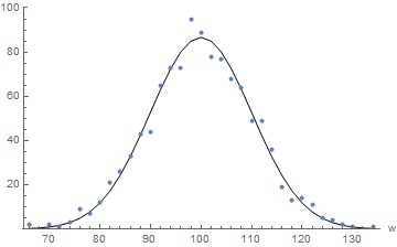
Actual vs Predicted Frequencies (Wealth After 100 Iterations, 1089 Agents)
Autonomy
Agents
Recall that this course uses the term agent for any actor in the conceptual model. The important thing about an agent is that, in the conceptual model, it is understood as a source of actions. For example, our gamblers bet; we understand them as a source of betting actions. The understanding places no constraints on how agents may be implemented in software. It is an extremely unrestricitve use of the term agent, and more restrictive uses are common. This section explores some additional properties we might expect agents to have. One of these properties is autonomy.
Behavior and Autonomy
We can trace the word autonomy via Greek roots to the concept of having authority over oneself. That is, the determinants of one’s behavior are at least partly internal, not entirely external. An agent is autonomous to the extent that it can be understood as determining its own behavior without any external direction. What this might mean metaphysically can be philosophically perplexing, and when applied to simulation modeling this appears particularly problematic. Software agents always act in accord with their programming, so to that extent they must always be subject to external direction.
Nevertheless, we will give a very simple meaning to autonomy in the context of agent-based modeling. This section introduces a notion of minimal autonomy suitable for agent-based modeling and simulation.
Minimal Autonomy
To be minimally autonomous, the behavior of an agent must have some dependence on its own state or its own information about its environment. If an agent is at least minimally autonomous, we call it an autonomous agent. For now, we will emphasize state-dependent behavior. In this case, an agent has at least minimal autonomy if its behavior depends on its own state.
Our gamblers do not have even minimal autonomy.
A gambler has a single state variable: wealth.
It has a single behavior: bet.
In the very simple conceptual model presented above,
the betting behavior of a gambler does not depends in any way on its wealth.
A gambler is conceived as acting and is thereby an agent,
but this does not imply any autonmy.
Autonomy and Agency
Since our gambler agents have no autonomy, some authors would not even call them agents. The amount of autonomy required before an actor can be called an agent has been a matter of considerable debate. This course does not engage that debate. Agency is determined by our understanding action in the conceptual model, whether or not an action is autonomous.
Nevertheless, the actors in our conceptual models will often require at least minimal autonomy. Recall that an agent has minimal autonomy if its behavior depends on its own state. Later on we will be interested in agents whose behaviors clearly derive from underlying goals. We will consider such agents to be more strongly autonomous.
State-Dependent Behavior
When we introduced our concept of a minimal agent, we specified that an agent must be capable of behavior can affect some values of its attributes. We introduce autonomy when an some agent depends in some way on some values of its attributes.
So far, our gambler agent has a single behavior: bet.
However, this behavior does not yet depend on the agent’s wealth.
For example, a gambler will continue to gamble even if wealth becomes negative.
When we say a model is agent-based, we usually mean that some agents are at least minimally autonomous in the following sense: we understand each agent as responding at least in part to its own state when selecting actions from its feasible set. Let us modify our gambler agents by introducing the following very simple dependence of behavior on state: a gambler will gamble only if wealth is positive. One way to achieve this is by conditional branching.
Conditional Branching
A condition is an expression that evaluates to true or false.
(We sometimes call this a binary or boolean condition.)
A branch is a code block that may be executed or skipped.
We use the term conditional branching to indicate
that the execution of a branch depends on the value of a condition.
Programming languages typically provide branching constructs
that allow us to implement conditional branching.
For example,
we might modify our conceptual model to include
a restriction that only gamblers with positive wealth are able place bets.
To implement this change in our simulation model,
we might modify our bet procedure,
adding a condition that tests for positive wealth:
wealth > 0.
Illustrate conditional branching by
moving the code for placing a bet into a branch,
so that it is executed if this condition is satisfied.
Call the resulting procedure bet01.
NetLogo Braching: The if Statement
The basic branching construct in NetLogo
is the if statement.
Again using angle brackets to indicate where
we need to substitute actual code,
we can charaterize the if statement as
if <condition> [<commands>]
Based on this syntax,
we can change our bet procedure
to condition on positive wealth.
As a visual aid, put the condition in parentheses.
(This is not required by NetLogo.)
The choice of indentation is also entirely optional.
However, as usual,
the brackets enclosing the commands are required to create a command block.
The command block will be executed if the condition evaluates to true.
Autonomy as State-Dependent Behavior
Betting behavior now depends on the agent’s current wealth. Each gambler examines its current wealth and, based on this wealth, determines whether to place a bet. This dependency of the agent’s behavior on its own state is a example of minimal autonomy. Each agent determines, based on its own state and without any external direction, whether or not to place a bet.
Autonomy: Conceptualization vs Implementation
Nevertheless, our notion of autonomy is conceptual. It does not imply any particular implementation in code. To help make this observation more concrete, consider the following three implementations of the betting stage in our simulation.
Ask every gambler to run
bet01.Ask every gambler to run
bet, if it has positive wealth.Determine which gamblers have positive wealth, and ask them to run
bet,
These three betting-stage implementations evidentally lead to the same outcomes. One can imagine an argument that the the agent is more autonomous in the first case, but that is not the view in this course. We consider the difference between these three approaches to be no more than an implementation detail that has no effect on the conceptual autonomy of our agents. This is true even if we pre-filter the agents for positive wealth. In our gambling simulations, all three implementations will produce the same outcomes. They are three different ways to implement a conceptual model in which the agents have minimal autonomy.
NetLogo: Three Implementations of Conditional Betting
Here are the first two implementation.
ask patches [bet01]

ask patches [if (wealth > 0) [bet 1]]
NetLogo provides the with primitive for filtering of agentsets.
We can get all the patches with positive wealth as
patches with [wealth > 0].
So the following code is yet another way to produce the same outcomes,
with no implications for our understanding of the autonomy of our agents.
ask patches with [wealth > 0] [bet 1]
This last implementation is perhaps the most common idiom for NetLogo programmers,
for reasons that we will explore in later lectures.
However, the expression patches with [wealth > 0] creates a new agentset,
which consumes computational time and memory.
In very large models,
such computational concerns can become important.
We will return to these issues in later lectures.
Autonomous Agents
Although the previous section developed a multi-agent simulation, most practitioners would not consider it to be an agent-based model. Two important reasons for this are the following:
inadequately autonomous agents
lack of interaction among agents
Adding conditional betting to the model made the agents minimally autonomous. Howevr, they still do not interact. Models are considered to be agent-based when the outcomes of interest result from the repeated interaction of autonomous actors with their environment (which includes other actors). Therefore, for a model to be considered to be agent-based, some agents must be at least minimally autonomous and responsive to some aspect of their environment (which includes other agents).
Responsive Agents
We have explored how to create simple agents that have:
state (i.e., attributes)
heterogeneity (i.e., differences in state)
behavior
minimal autonomy (i.e., behavior depends on state)
In our multi-agent simulation, our agents are heterogeneous: they develop diverse values of wealth. An agent whose betting behavior depends on its wealth is minimally autonomous. Yet a simulation with such agents is still not generally considered to be agent-based, because the behavior of the agents does not respond to the external environment. A minimal agent-based model must include:
agents that can acquire information from their environment
some dependence of agent behavior on this information
We will need to elaborate these concepts. One might say that a gambler who bets experiences wins and losses, which is information about the betting environment. However, our notion of acquiring information from the environment will be more demanding than this. However, if the gambler recorded a history of wins and losses and based betting on the estimated the probability of a win, this would indeed be reactive behavior.
We will classify responsive behavior as reactive or interactive. Reactive behavior responds to information about the environment, including information about other agents. Interactive behavior targets other agents in the model.
Agent Environment
In this course, the notion of an agent’s environment is extremely flexible. It may simply be constituted by the other agents, or conceptually there may also be an institutional or even a physical environment that agents interact with. The agents we have considered so far do not interact with their environment, because behavior does not depend on information about the environment. Interaction with the environment is a core feature of agent-based models.
The incorporation of interaction in a conceptual model substantially increases the complexity of the agents. In order to meaningfully interact with the environment, an agent must be able to acquire information from its environment and alter its behavior in response to this information. For example, up to now our gamblers have been implicitly playing against the house, perhaps by putting coins in a simple slot machine. Interacting gamblers might gamble with each other. Often the existence of interaction requires the model to include rules of agent interaction.
In terms of implementing more complex conceptual models as simulation models, this course will slowly increase the complexity of agent interactions. That will be a core project of upcoming lectures, and it will be a key step in moving us towards agent-based social science.
Summary and Conclusions
What Is An Agent?
An agent is often a stylized representation of a real-world actor:
either an individual, such as a consumer or entrepreneur,
or an aggregate of individuals,
such as a corporation or a monetary authority
(which may in turn be explicitly constituted of agents).
This lecture works with a single type of agent:
the Gambler.
Our understanding of agency is rooted in the conceptual model. Any actor in the conceptual model is an agent. Each agent has:
attributes
one or more rules of behaviour
Attributes may be very simple.
A Gambler agent only has a wealth attribute.
(Later we will care about multiple attributes
that together character an agent’s state.)
Behavior may also be very simple.
A Gambler agent only has a bet behavior,
and this behavior does not even depend on the gambler’s wealth.
(Later we will care complex behaviors that depend
on the agent’s state.)
Roughly, an agent’s behavior can be understood as reflecting underlying goals,
which may be implicit or explicit in the model.
The more explicit the goals are,
the easier it is to understand the agent as an actor in the model.
The goals of a Gambler agent are entirely implicit:
the conceptual model states that a gambler bets,
but it does not offer an reasons for this betting behavior.
Simple Agents
By definition, an agent-based simulation model requires more than this of its agents. For a simulation model to be agent-based, the actors in the model must pass the simple-agent hurdle. A simple agent is at least minimally autonomous and reactive.
In this course when we speak of an agent-based model, the presumption is that we are working with simple agents. We will occasionally consider more complex agents, which are pro-active, or have social ability, or may have additional capabilities as well.
What Is ABMS?
Our multi-agent gambling simulation is not considered to be an agent-based simulation because it lacks key features. At a minimum, an agent-based simulation model must include:
multiple heterogeneous agents
minimally autonomous agents
reactive or interactive behavior (i.e., a response to changes in the simulation environment)
The gambling simulation includes multiple heterogeneous agents, because each gambler has its own level of wealth. But these gamblers are not even minimally autonomous, because a gambler’s behavior does not depend on its state. Additionally, a gambler agent’s behavior is neither reactive or interactive. It does not respond to changes in the simulation environment.
Multi-Agent Gambling Model: Still Not Agent-Based
Our original gambling model was based on one simple agent, with an attribute and behavior. When we use only a single agent, we generally do not call the model “agent-based”. A model is ordinarily considered agent-based only if it involves multiple agents.
We then ran a simulation with many gamblers, where each each gambler gambled. This multi-agent simulation would usually still not be considered an agent-based model. Two reasons are the lack of interaction between agents and their environment and the lack of agent autonomy.
A model with a single agent in it will not generally be considered agent-based. A model with multiple agents that have no interaction will generally not be considered agent-based.
Agent Interactions in ABMS
In an ABM, a population of software objects is instantiated. The agents are then permitted to interact directly with one another. A macrostructure emerges from these interactions.
Each agent has:
certain internal states (e.g., preferences, endowments) and
rules of behaviour (e.g., seek utility improvements).
More complex agents may derive their rules of behavior from their goals. For example, a consumer agent may try to maximize utility.
Realism
One specific hope is that simulations will advance social science by enabling the creation of more realistic models. For example, economists can build models that incorporate important historical, institutional, and psychological properties that "pure theory" often has trouble accommodating, including learning, adaptation, and other interesting limits on the computational resources of real-world actors. Another specific hope is that unexpected but useful (for prediction or understanding) aggregate outcomes will emerge from the interactions of autonomous actors in agent-based simulations. These hopes are already being met in many surprising and useful ways [bonabeau-2002-pnas].
Complex Agents?
How complex should we make the agents in an agent-based model. There are many opinons about this but no single view. For North and Macal (2007), real agents can learn and adapt. They call agents lacking these features “simple agents” or “proto-agents”. We will essentially invert this by calling agents that can learn and adapt complex agents. Complex agents may also be capable of structured communication. For the most part, the present course will not make use of complex agents. However we will discuss strategy evolution, which is closely related to adaptation and learning. We will also allow behavior to depend on memory, which is again closely related to adaptation and learning.
Beyond Simple Agents
A minimal agent has attributes and behavior that depends on these attributes. In the context of agent-based modeling, a minimal agent must acquire information from the environment (possibly including the other agents) and respond to it.
The design of simulation agents should reflect an underlying conceptual model. Unfortunately, it is much easier to mutliply the features we would like agents to have than to implement these features. [Gilbert-2007-Sage]_ offers a fairly simple set of desired attributes:
Perception: can perceive their environment, possibly comprising other agents
Performance: a set of behaviours, such as:
Communication: can send and receive messages with each other
Action: can interact with the environment (eg. pick up food)
Motion: can move in the space
Memory: can remember their previous states, perceptions, and actions
Policy: a set of rules that determines how they will act, given their state and history
This is pretty close to our understanding of a minimal agent in an agent-based model. The big difference is the inclusion of memory, but in fact this is absent in many agent-based models.
Further agent features:
(Epstein 1999):
heterogeneity: not representative but may differ
local interactions: in a defined space
non-equilibrium dynamics: large-scale transitions, tipping phenomena (Gladwell 2000)
boundedly rational (Simon): information, memory, computational capacity
Agents of the Future?
Gilber and Troitzsch (2005) suggest eight desired attributes of agents, which far exceed the attributes of the agents.
- Knowledge & beliefs:
Agents act based on their knowledge of the environment (including other agents), which may be faulty --- their beliefs, not true knowledge.
- Inference.
Given a set of beliefs, an agent might infer more information.
- Social models.
Agents, knowing about interrelationships between other agents, can develop a social model, or a topology of their environment: who's who. etc.
Desired Attributes ...
- Knowledge representation.
Agents need a representation of beliefs: e.g. predicate logic, semantic (hierarchical) networks, Bayesian (probabilistic) networks.
“[Sebastian] Thrun [leader of the winning team in the 2005 DARPA Grand Challenge] had a Zen-like revelation: ‘A key prerequisite of true intelligence is knowledge of one's own ignorance,’ he thought. Given the inherent unpredictability of the world, robots, like humans, will always make mistakes. So Thrun pioneered what's known as probabilistic robotics. He programs his machines to adjust their responses to incoming data based on the probability that the data are correct.”
—Pacella (2005).
Desired Attributes ...
- Goals
Agents driven by some internal goal, e.g. survival, and its subsidiary goals (food, shelter). Usually definition and management of goals imposed on the agent.
- Planning.
Agent must (somehow) determine what actions will attain its goal(s). Some agents modelled without teleology (simple trial-and-error), others with inference (forward-looking), or planning.
- Language.
For communication (of information, negotiation, threats). Modelling language is difficult. (Want to avoid inadvertent communication, e.g. through the genome of a population in the GA.)
- Emotions.
Emergent features? Significant in modelling agents? Or epiphenomenal?
Summary and Conclusions
Explorations
Agency: Redo the single-agent simulation of this lecture by making
wealthis a global variable and implementingbetas a procedure that mutates this variable.Does this alternative implementation of the conceptual model change any results? Where is the agent in this implementation?
Hint: the notion of agency belongs to the conceptual model. The conceptual agent guides the computational implementation, but there is no requirement that a conceptual agent be represented by a particular object in the simulation.
Betting: Write the
betprocedure so that it accepts a parameter, the amount bet. Each time an agent bets, the amount bet is either forfeit or doubled, with equal probability.Parameters: After completing the previous exercise, add sliders for the amount bet and the initial wealth of an agent. Predict the changes in simulation outcomes that you will see if you double both of these model parameters. Run the simulation to test your prediction.
Random Walk: Implement our single-gambler simulation with \(100\) iterations. Add a plot to the NetLogo
Interfacetab, and plot the evolution of the gambler’s wealth over time. Repeat the simulation several times: does the plot always look the same?Plotting: Edit the ranges on the plots in our gambling simulation to be more aesthetic. (E.g., so that the plot of mean wealth lies nearer to the center of the plot region.)
Autonomy: Introduce a positive wealth constraint: gamlbers only bet when they have positive wealth, How do the simulation outcomes change after 100 iterations? How do the simulation outcomes change after 1000 iterations? If the change depends on the number of iterations in the simulation, explain why.
Stopping Criterion: Run the multi-agent gambling simlation with a positive wealth constraint until a quarter of all agents have zero wealth. How long does this take the first time you try it? How long does this take on average?
Further Reading
David Bowen’s Classroom Computer Models uses NetLogo to explore physics http://www.is.wayne.edu/DRBOWEN/Class-Room_Models/
References
Bonabeau, Eric. (2002) Agent-based Modeling: Methods and Techniques for Simulating Human Systems. Proceedings of the National Academy of Sciences 99, 7280--7287.
Coleman, James S. (1986) Social Theory, Social Research, and a Theory of Action. American Journal of Sociology 91, 1309--1335.
Gilbert, Nigel, and Klaus Troitzsch. (2005) Simulation for the Social Scientist. : Open University Press.
Krakauer, David, et al. (2020) The Information Theory of Individuality. Theory in Biosciences 139, 209--223. https://doi.org/10.1007/s12064-020-00313-7
North, Michael J., and Charles M. Macal. (2007) Managing Business Complexity: Discovering Strategic Solutions with Agent-Based Modeling and Simulation. : Oxford University Press.
Raub, Werner, Vincent Buskens, and Marcel A. L. M. Van Assen. (2011) Micro-Macro Links and Microfoundations in Sociology. The Journal of Mathematical Sociology 35, 1--25. https://doi.org/10.1080/0022250X.2010.532263
Wilensky, Uri. (1999) "NetLogo". Center for Connected Learning and Computer-Based Modeling. Northwestern University . http://ccl.northwestern.edu/netlogo
Wilensky, Uri, and William Rand. (2015) An Introduction to Agent-Based Modeling: Modeling Natural, Social, and Engineered Complex Systems with NetLogo. Cambridge, MA: MIT Press.
Copyright © 2016–2023 Alan G. Isaac. All rights reserved.